A Two way Algorithm Method for Mining of
Frequent Itemsets Using MapReduce
B Revathi Lavanya MIAENG
N Sameera
J.Malathi
Assistant Professor Assistant Professor Assistant Professor
CVR College of Engineering Sir CRR collegeof Engineering Sir CRR college of Engineering
Abstract—Existing mining algorithms for frequent itemsets lack a mechanism that enables automatic parallelization, load balancing, data distribution, and fault tolerance on large clusters. As a solution to this problem, we design a two step algorithm method for mining of frequent itsemsets using the MapReduce programming model. To achieve minimum running time for the corresponding minimum support, FP growth algorithm is used. This paper incorporates the mining of frequent items using FP trees. Also three MapReduce jobs are implemented to complete the mining task. In the crucial third MapReduce job, the mappers independently decompose itemsets, the reducers perform combination operations. To optimize the mining process and to measure load balance across the cluster’s computing nodes FiDoop-HD, an extension of FiDoop is used, to speed up the mining performance for high-dimensional data analysis. Extensive experiments using real-world celestial spectral data demonstrate that our proposed solution is efficient and scalable.
Index Terms—Frequent itemsets, minimum support,frequent items FP tree, Hadoop cluster, load balance, MapReduce.
I.INTRODUCTION
Due to the excessive volumes of data generated everyday frequent itemsets mining (FIM) is a core problesm in association rule mining (ARM), sequence mining. Since FIM takes high computation and input-output intensity , FIM should be made much faster since it plays a significant role in mining.
As existing algorithms running on a single machine suffer from performance deterioration. To address this issue, we investigate how to perform FIM using MapReduce—a widely adopted programming model for processing big datasets. In this paper distribution of large data across clusters to balance load is described thereby optimizing the performance of FIM. FIM process is categorized as two algorithms namely, Apriori and FP-growth schemes. Apriori is a classicalgorithm using the generate-and-test process that generates a large number of candidate itemsets; Apriori has to repeatedly scan an entire database.To reducethe time required for scanning databases an approach involving FP-growth and FiDoop HD was proposed, which avoids generating candidate itemsets. Most previously developed FIM process iscategorized as two algorithmsnamely Apriori and FP-Growth schemes.priori is a classic algorithm using the generate and test process that , which avoids generating candidate itemsets. Most previously developed FIM algorithms were built upon the Apriori
algorithm.Unfortunately, in Apriori-like FIM algorithms, each processor has to scana database multiple times and to exchange an excessive number of candidate itemsets with other processors. Therefore, Apriori-like FIM solutions suffer potential problems of high I/O and synchronization overhead.The scalability problem has been addressed by the implementation of a handful of FP-growth and FiDoop-HD. Rather than considering Apriori ,we incorporate the FP tree in the design of our FIM technique. The basic idea of FP growth algorithm is to remove infrequent items through recursive elimination procedure at the same time deleting these infrequent transactions. This means they do not appear in the user specified minimum number of transactions. The four advantages of FP growth algorithm are : 1)only two passes over data set 2) compresses data set 3)no candidate generation 4) much faster than Apriori algorithm.
More importantly, the existing algorithms lack a mechanism that enables automatic parallelization, load balancing, data distribution, and fault tolerance on large computing clusters. To solve the aforementioned open problems, we use a parallel FIM algorithm called FiDoopHD using the MapReduce program-ming model. Compared with the existing frequent items FP tree algorithm, FiDoopHD has distinctive features. In FiDoopHD, the mappers independently and concurrently decompose itemsets; the reducers perform combination operations.
We use FiDoopHD on our in-house Hadoop cluster. We observe that data partitioning and distribution are critical issues in FiDoop, because itemsets with different lengths have various decomposition and construction costs. To optimize the performance of FiDoop, we used a new data partitioning method to well balance computing load among the cluster nodes; FiDoop-HD, an exten-sion of FiDoop, to meet the needs of high-dimensional data processing.
The main contributions of this paper are summarized as follows.
1) We made a complete overhaul to FP tree.
2) We used the frequent itemsets mining method FiDoopHD using the MapReduce programming model. 3) We proposed FP growth algorithm for the first two
4) We used FiDoopHD algorithm for the third Map-Reduce job to improve performance for the high dimensional datasets.
5) We conducted extensive experiments using a wide range of synthetic and real-world datasets, and we show that combination of FP growth and FiDoopHD algorithms is efficient and scalable on Hadoop clusters.
II.PRELIMINARY
In this section, we first briefly review association rules. Then, we summarize the basic idea of the FP growth algorithm along with its core data structures.
A. Association Rules
ARM provides a strategic resource for decision support by extracting the most important frequent patterns that simulta-neously occur in a large transaction database. A typical ARM application is market basket analysis. An association rule, for example, can be “if a customer buys X and Y, then 90% of them also buy Z.” In this example, 90% is the confidence of the rule. Apart from confidence, support is another measure of asso-ciation rules, each of which is an implication in the form of A⇒ B . Here, A and B are two itemsets, and A∩B =∅.The confidence of a rule A⇒ B is defined as a ratio between support(A∪B) and support(A). Note that, an item-set A has support s if s% of transactions contain the itemset. We denote s= support(A); the support of the rule A⇒B is support(A∪B).The ultimate objective of ARM isto discover all rules that satisfy a user-specified minimum support and minimum confi-dence. The ARM process can be decomposed into two phases: 1) identifying all frequent itemsets whose support is greater than the minimum support and 2) forming conditional impli-cation rules among the frequent itemsets. The first phase is more challenging and complicated than the second one.
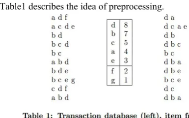
B. FP Preprocessing
The following are the steps of FP Preprocessing: 1)In the first scan the frequent item sets are determined. 2)All the infrequent itemsets are deleted from the transaction as they never be part of a frequent item set.
3)All the frequent item sets that are determined are arranged in the descending order with respective to their frequency. 4)The above steps is performed since it optimizes the execution rather than the frequent itemsets being arranged in random or ascending order.
Table1 describes the idea of preprocessing.
C. FP Tree
After all individually infrequent items have been deleted from the transaction database, it is turned into an FP-tree , which is basically a prefix tree for the transactions That is, each path represents a set of transactions that share the same prefix, each node corresponds to one item.
In addition, all nodes referring to the same item are linked together in a list, so that all transactions containing a specific item can easily be found and counted by traversing this list which can be accessed through a head element, that states the total number of occurrences of the item in the database. Figure 1 shows the FP-tree for the (reduced) database shown in Table 1.The head elements of the item lists are shown to the left of the vertical grey bar, the prefix tree to the right of it. Figure 1 showes the fp-tree.
The FP tree concept is explained with an example below:
The initial FP-tree is built from a main memory representation of the (preprocessed) transaction database as a simple list of integer array and the resultant list is sorted lexicographically, whereas this list is converted into an FP tree with intensive recursive procedure with depth k, the kth item in each transaction is used to split the database into sections, one for each item. For each section a node of the FP-tree is created and labeled with the item corresponding to the section and in turn it is processed recursively, which is again split into subsections,. Finally a new layer of nodes (one per subsection) is created .
processed at a time, only the FP-tree representation and one new transaction is in main memory. This usually saves space, because an FP-tree is often a much more compact representation of a transaction database.
D. Projecting and Pruning FP Tree
The core operation of the FP-growth algorithm is to compute an FP-tree of a projected database containing transactions with specific items. The FP-growth
algorithm contains two different projection methods. Both the methods start processing from copying certain nodes of the FP tree which are identified by the very deepest level of the FP tree , thus in turn produces the shadow of the same .Now the copied nodes are then linked and detached from the original FP-tree, yielding an FP-tree of the projected database.
Figure2
Later on the deepest level of the original FP-tree, which corresponds to the item on which the projection was based, is removed, and the next higher level is processed in the same way. These two projection methods are mainly in the order in which they traverse and copy the nodes of the FP-tree. In the Figure3 , the red arrow represents the processing and blue arrow represents the projection FP-tree is the created projection. Below figure 3 depicts the first method of projection of FP tree.
In an outer loop, the lowest level of the FP-tree, that is, the list of nodes corresponding to the projection item, is traersed and for each node of this list, the parent pointers are followed to traverse all ancestors up to the root. Each encountered ancestor is copied and linked from its original(this is what the auxiliary pointer in each node, which was mentioned above, is needed for).
During the copying, the parent pointers of the copies are set, the copies are also organized into level lists, and a sum of the counter values in each node is computed in head elements for these lists.
Figure3:first stage of projection
In a second traversal of the same branches, carried out in exactly the same manner where in which the copies are detached from their originals (the auxiliary pointers are set to null), which yields the independent projected FP-tree which is processed repeatedly by considering a prefix.
The projection in the second phase traverses in an outer loop which is the deepest level of the FP tree. It also copies the parent of each node, not its higher ancestor, making it possible to find the ancestors in later steps.After projection , pruning is performed on the FP tree , which further remove some infrequent item sets. This pruning is achieved by traversing the levels of the Fp tree from top to bottom.
E. MapReduce Framework
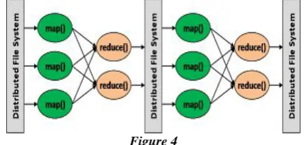
MapReduce is a promising scalable programming model for data-intensive applications and scientific analysis. A MapReduce program expresses a large distributed computation as a sequence of parallel operations on datasets of key/value pairs. A MapReduce computation has two phases, namely, the Map and Reduce phases. MapReduce greatly improves programmability by offering automatic data management, highly scalable, and transparent fault-tolerant processing. Also, MapReduce is running on clusters of cheap commodity servers—an increasingly attractive alternative to expensive computing platforms. The Mapper splits the input data into a large number of fragments, which are evenly distributed to Map tasks across the nodes of a cluster to process .Each Map task takes in a key-value pair and then generates a set of intermediate key-value pairs. After the MapReduce runtime system groups and sorts all the intermediate values associated with the same intermediate key, the runtime system delivers the intermediate values to Reduce tasks. Each Reduce task takes in all intermediate pairs associated with a particular key and emits a final set of key-value pairs. Both input pairs of Map and the output pairs of Reduce are managed by an underlying distributed file system called HDFS
This picture would depict the process of map and reduce functionality more clearly
Figure 4
This figure4 describes that data taken from the distribute file system is given as an input to the mapper which after computation generates the output which is in turn given as input to the reducer. When the dimensionality is huge or large then we consider distributed file system as single system may not support such a huge data. So when multiple systems are part of this distributed file system then many mappers would function or process the data from database. As part of this paper we suggest that the first two phases of scan would involve the two Map-Reducer programs running on the FP-growth algorithm. But the third map-reduce program would purely run on the Fidoop HD algorithm concepts. Since FidoopHD optimizes the third map reduce computations effectively. The below graphs depicts the performance of FP , FiDoop,FiDoopHD algorithm with respective to the data size.
Similarly when considered the minimum support definitely there would be change in the performance of all the three algorithms i.e FP, FiDoop, FiDoopHD
The same can be viewed by the below graphs.
Graph1
FiDoop,FiDoopHD algorithm with respect to the data size. Similarly when considered the minimum upport definitely there would be change in the performance of all the three algorithms :FP, FiDoop, FiDoopHD.
III. OVERVIEW
The three Map Reducer programs are explained below : 1. The first mapper program would mine the transaction
database by removing infrequent sets.This output from the map is given to reducer as an input which would order the frequent itemsets in descending order and would build a FP tree.
2. The second map programs takes the FP tree generated by the first reducer and would perform the projection operation by generating a projection FP tree. This output is taken by the second reducer program which would perform the pruning process and by removing again some infrequent itemsets.
3. The above two phase 1) and 2) are performed using FP growth algorithms.
4. The third map - reducer program takes the output from the second reducer , which would recursively processes the data and generates a minimum 2 Item sets using the FiDoopHD algorithm.
The FP growth algorithm is as follows
A.First Map - Reduce Algorithm Input: minsupport, DBi;
Output: FP tree
1. function MAP(key offset, values DBi)
2. //T is the transaction in DBi
3. for all T do
4. items ←spliteach T;
5. for all item in items do
1. count++
2. end for
6. output( item, count);
7. end for 8. end function
10. reduce input: (itemset,count )
11. function REDUCE(key item, values count)
12. Items=sort(itemset,count) /*sorts the items in descending order*/
13. fptree_generation(items); /*generates FP tree */
14. end function
B.Second Map-Reduce Algorithm Input: minsupport, DBi;
Output: FP Tree after Projection and Pruning 1. function MAP(FP_Treei)
2. //T is the deepest level node in FP Tree
3. /* The below for loop would project the FP Tree */ 4. for all (T) do
4. new_nodes=choose(T); 5. detach(FP Tree,new_nodes)
6. FP_Tree=create_shadow(new_nodes,FP_Tr ee)
7. output(FP_Tree)
8. end for
9. end function
14. function REDUCE(FP_Tree)
15. FP_Tree=remove(FP_Tree,minsupport) 16. List=create_list(FP_Tree);
17. output(List) /*The output from this function is List */
C.Third Map Reduce Algorithm
Input: List, Output:-FP Tree
1. function MAP(List) 2. // M is the size of the List 2. for all (k is from M to 2) do 3. for all (k-itemset in List) do
4. decompose(k-itemset, k-1, (k-1)-itemsets); /*Each k-itemset isonly decomposed into (k-1)-itemsets */
5. (k-1)-file ← the decomposed (k-1)-itemsets 6. union the original (k-1)-itemsets in (k-1)-file;
2. for all (t-itemset in (k-1)-file) do
3. t -FP-tree←t-FP-tree generation(local-FPtree,t-itemset);
8. output(t, t-FP-tree);
9. end for
10. end for 11. end for 12. end function
D.Algorithm 4 Generate itemsets: To Generate All k-itemsets by Pruning the Original Database
Input: minsupport, DBi; Output: k-itemsets;
1. function MAP(key offset, values DBi) 2. //T is the transaction in DBi 3. for all (T) do
4. items ←spliteach T;
5. for all (item in items) do
6. if (item is not frequent) then 4. prune the item in the T;
8. end if
9. k-itemset ←(k, itemset) /*itemset is the set of frequent
items after pruning,
10. whose length is k */
10. output(k-itemset,1);
11. end for
12. end for
13. end function
14. function REDUCE(key k-itemset, values 1)
15. sum=0;
16. for all (k-itemset) do
17. sum += 1;
18. end for
19. output(k, k-itemset+sum);//sum is support of
this itemset end function
we pay particular attention to the third MapReduce job, which is a performance bottleneck of the FiDoop algorithm.
IV. SUPPORTING DETAILS A. Load Balance
The decompose() function of the third MapReduce job accomplishes the decomposition process. If the length of an itemset is m, the time complexity of decomposing the
item-set is O(2
m
). Thus, the decomposition cost is exponentially proportional to the itemset’s length. In other words, when the itemset length is going up, the decomposition overhead wi. Wigives rise to poor load-balancing performance .Weintroduce the entropy measure as a load balancing metric. Load is perfectly balanced across all the nodes.If WB(D) equals to 0 (i.e., WB(D)= 0), decomposition load is concentrated on one node.
All the other cases are represented by 0 < WB(D) < 1. We experimentally evaluate the load-balancing performance. B. High- Dimensional Optimization
The aforementioned analysis confirms that if the length of itemsets to be decomposed is large, the decomposition cost will exponentially increase. In this section, we conduct experiments to investigate the impact of dimensionality on FiDoop. We also compare FiDoop with a popular solution parallelization of FP-growth (Pfp) . We presents an optimization algorithm called FiDoop-HD for high-dimensional data processing.
When it comes to mining frequent itemsets, varying dimensionality leads to a wide range of item set lengths. Our algorithm needs to decompose each itemset generated by pruning infrequent items for each transaction.Graph 2 shows the impact of dimensionality on the processing time of the tested algorithms. We made use of the series of D1000W, which are described in detail (see Synthetic Dataset). In the group of experiments, the number of transactions is 10 000 000 and the average transaction size is anywhere between 10 and 50.
Graph 2: Effect of dimensionality on different algorithms (on four nodes). Comparison of (a) FiDoop and Pfp and (b) FiDoop-HD and.Pfp
V. FIDOOP-HD
FiDoop-HD decomposes the list of itemsets in a decreasing order of itemset length. After reading M-itemsets from a cache file, FiDoop-HD decomposesthe M-itemsets into a list of (M− 1)-itemsets. Note that, M is the maximal length of itemsets. Then, these itemsets combine original (M− 1)-itemsets to be stored.
Algorithm 5 FiDoop-HD-MiningMap: High-DimensionalOptimization for Map() Function
Input: k-file /*k-file(2≤k≤M) is used to store the frequent k-itemsets generated in the second MapReduce.*/
Output: (k-1)-Fp-tree
1. function MAP(key k, values k-file) 2. for all (k is from M to 2) do 3. for all (k-itemset in k-file) do
4. decompose(k-itemset, k-1, (k-1)-itemsets); /*Each k-itemset isonly decomposed into (k-1)-k-itemsets */
5. (k-1)-file ← the decomposed (k-1)-itemsets union
the original (k-1)-itemsets in (k-1)-file;
6. for all (t-itemset in (k-1)-file) do
7. t − Fp − tree ←t-Fp-tree
generation(local-Fp-tree, t-itemset);
8. output(t, t-Fp-tree);
9. end for
10. end for
11. end for
12. endfunction
decompose k-itemset into (k− 1)-itemsets rather than into two-itemsets.In case of multi-ple files stored on a data node, the node sequentially loads and processes the files.
The cost of decomposing an m-itemset into (m− 1)-itemsets can be modeled as c mm−1. Given a file storing all itemsets
whose length is m, the decomposition cost of the file is C(ISm)×c
m
m−1, where C(ISm) is the count of ISm in the
file. Hence, the time complexity of the entire process can be approximated as max(C(ISi))×(cMM−1+cMM−−21+· · ·+c23), which
can be further written as max(C(ISi))×(M×(M+ 1)/2), 2
<i≤M.
It is essential and critical to address the I/O performance issues in FiDoop-HD due to the following reasons. First, itemsets decomposed in the previous stages have to be saved in new files for subsequent phases. Second, FiDoop-HD does inherently incorporate a load-balancing policy, because each node processes the files storing itemsets with an identical length.
VI MINIMUM SUPPORT:
Minimum support plays an important role in mining frequent itemsets. We increase minimum support thresholds from 0.0001% to 0.0003% with an increment of 0.00005%, thereby evaluating the impact of minimum support on Pfp and our proposed algorithms containing three MapReduce jobs using both celestial spectral and synthetic dataset
the performance of the evaluated algorithms. This is because an increasing number of items satisfy the small minimum support when the minsupport is decreased; it takes an increased amount of time to process the large number of items. We also observe from Graph. 3(a) that the proposed algorithms are superior to Pfp in processing the low-dimensional dataset. When it comes to the high-dimensional dataset [see Graph. 3(b) and (c)], FiDoop-HD behaves optimally and FiDoop shows its downside. These performance trends are reasonable, because the decomposition cost of FiDoop will exponentially increase, which in turn
gradually offsets the gain in mining capacity with the increase of the item-set length. It is evident from these experimental results that FiDoop-HD improves the performance of FiDoop in the case of high-dimensional datasets. This observation is consistent with those drawn from Graph. 3(d)–(f), which show the running time of the three stages of FiDoop, FiDoop-HD, and Pfp on celestial spectral dataset. Although Pfp is seemingly superior to FiDoop in running time when high-dimensional datasets are processed, Pfp’s space consumption and the shuffling cost in the parallel process are higher than those of our solution. As a result, FiDoop-HD’s performance is better than that of Pfp. Graph 3(d) and (e) reveals that the running time of the first and second MapReduce jobs in FiDoop and FiDoop-HD are insensitive to minimum support. The mappers in FiDoop and FiDoop-HD have to scan the entire dataset and the reducers combine the output produced by the mappers; a similar case applies for the first MapReduce job of Pfp [see Graph. 3(f)]. Interestingly, the running times the third MapReduce job of our algorithms and the second MapReduce job of Pfp sharply increase with the decreasing value of minimum support. A small minimum support gives rise to an increasing number of k-itemsets to be decomposed by the third MapReduce job. For the Pfp case, the time spent in grouping and processing FP-tree goes up as the number of k-itemsets increases.
E. Speedup
We evaluate the speedup performance of Pfp, FiDoop, and FiDoop-HD by increasing the number of data nodes in the test Hadoop cluster from 4 to 16 with an increment of 2. The celestial spectral dataset is applied to drive the speedup analysis of the three algorithms.
Th results illustrated in Graph4 show that the speedups of the three algorithms scale linearly when the number of data nodes increases from 4 to 14. When the num-ber of data nodes is further increased from 14 to 16, the speedup improvement marginally slows down. Such a speedup trend can be attributed to the fact that increasing the num-ber of data nodes under a fixed input data size inevitably: 1) reduces the amount of itemsets being handled by each node and 2) increases communication overhead between mappers and reducers.
Graph 3. Effect of minimum support on (a) 10 dimensions, (b) 40 dimensions, (c) celestial spectral dataset, (d) three stages of FiDoop, (e) three stages of FiDoop-HD, and (f) three stages of Pfp.
There is a slowdown in speedup improvement and the rea-son is twofold. First, each node has to load input itemsets from the HDFS; such input load has more noticeable impacts on FiDoop-HD than on FiDoop.
Graph 4:Speedup performance
In this group of experiments, we evaluate the scalability of FiDoop when the size of input dataset grows dramatically. Graph 5 shows the running time of FiDoop and FiDoop-HD when we scale up and process the dimensionality of the series of D1000W.
Graph 5: Scalability of FiDoop and FiDoop-HD when the size of input dataset increases. The number of dimensions is set to 10
Graph 5 clearly reveals that the overall execution time of FiDoop and FiDoop-HD goes up when the input data size is sharply enlarged.
Graph 5 shows that when the dimension is rel-atively high, FiDoop-HD is superior to FiDoop in terms of execution time; More importantly, FiDoop-HD optimizes the performance of FiDoop for processing high-dimensional data; FiDoop-HD is superior to FiDoop when itemsets to be decomposed are large. Pfp is seemingly better than FiDoop when high-dimensional datasets are processed.
CONCLUSION
To solve the scalability and load balancing,fault tolerence challenges in the existing mining algorithms, we described a two step algorithm method for mining of frequent item set using the Map-Reduce model.Which contain two methods for efficiently projecting FP-tree with the help of fp growth algorithm. Fpgrowth seamlessly integrates first two MapReduce jobs and FiDoop-HD performs the complex third mapreduce job to accomplish miningof frequent itemsets because the third MapReduce job plays an important role in mining frequent items; its mappers independently decompose item-sets whereas its reducers construct them into small data sets.
We designed and implemented FiDoop-HD to efficiently handle high-dimensional data processing. FiDoop-HD decomposes the M-itemsets into a list of (M− 1)-itemsets, which are further decomposed into (M − 2)-itemsets to be unioned into the original (M − 2)-itemsets. This procedure is repeatedly carried out until the entire decomposition process is accomplished.
REFERENCES
1. Critian Borgelt “An implementation of the fp growth.department of language PROCESSING AND KNOWLEDGE ENGINEERING SCHOOL OF COMPUTER SCIENCE, Otto-von-Guericke-University of Magde burg Universitatsplatz¨ 2, 39106 Magdeburg, Germany.
2. C.L. Blake and C.J. Merz. UCI Repository of MachineLearning Databases. Dept. of Information and Computer Science, University of California at Irvine, CA, USA 1998
3. Pramudiono and M. Kitsuregawa, “FP-tax: Tree structure based generalized association rule mining,” inProc. 9th ACM SIGMOD WorkshopRes. Issues Data Min. Knowl. Disc., Paris, France, 2004, pp. 60–63.
4. R. Agrawal, T. Imielinski,´ and A. Swami, “Mining association rules between sets of items in large databases,” ACM SIGMOD Rec., vol. 22, no. 2, pp. 207–216, 1993.
5. Agrawal, H. Mannila, R. Srikant, H. Toivonen, and A. Verkamo. Fast Discovery of Association Rules. In: 307– 328