The development of an affinity evaluation and prediction system by using protein–protein docking simulations and parameter tuning

(1)

Advances and Applications in Bioinformatics and Chemistry

Dove

press

open access to scientific and medical research

Open Access Full Text Article _{O R i g i n A L R e s e A R C h}

The development of an affinity evaluation

and prediction system by using protein–protein

docking simulations and parameter tuning

Koki Tsukamoto1

Tatsuya Yoshikawa1,2

Kiyonobu Yokota1

Yuichiro hourai1

Kazuhiko Fukui1

1_{Computational Biology Research}

Center (CBRC), national institute of Advanced industrial science and Technology (AisT), Koto-ku, Tokyo, Japan; 2_{Department of Bioinformatic}

engineering, graduate school of information science and Technology, Osaka University, Toyonaka, Osaka, Japan

Correspondence: Kazuhiko Fukui Computational Biology Research Center (CBRC), national institute of Advanced industrial science and Technology (AisT), 2-42 Aomi, Koto-ku, Tokyo 135-0064, Japan

Tel +81 3 3599 8060 Fax +81 3 3599 8081 email [email protected]

Abstract: A system was developed to evaluate and predict the interaction between protein

pairs by using the widely used shape complementarity search method as the algorithm for docking simulations between the proteins. We used this system, which we call the affinity evaluation and prediction (AEP) system, to evaluate the interaction between 20 protein pairs. The system first executes a “round robin” shape complementarity search of the target protein group, and evaluates the interaction between the complex structures obtained by the search. These complex structures are selected by using a statistical procedure that we developed called ‘grouping’. At a prevalence of 5.0%, our AEP system predicted protein–protein interactions with a 50.0% recall, 55.6% precision, 95.5% accuracy, and an F-measure of 0.526. By optimizing the grouping process, our AEP system successfully predicted 10 protein pairs (among 20 pairs) that were biologically relevant combinations. Our ultimate goal is to construct an affinity database that will provide cell biologists and drug designers with crucial information obtained using our AEP system.

Keywords: protein–protein interaction, affinity analysis, protein–protein docking, FFT, massive parallel computing

Introduction

Proteins have diverse functions ranging from molecular machines to signaling. They participate in catalytic reactions, provide transport, form viral capsids, traverse mem-branes and construct regulated channels, transmit information from DNA to RNA, thus making it possible to synthesize new proteins. Given their importance, considerable effort has centered on the prediction of protein functions. A major way of achieving this is through the identification of binding partners. If we know the function of at least one of the components with which the protein interacts, that should enable us to determine its function(s) and the pathway(s) in which it plays a role. This holds since the vast majority of the functions performed by proteins in living cells involve protein–protein interactions (PPI).1,2_{Hence, by observing the intricate network of} these interactions we can map cellular pathways, their interconnectivities and their dynamic regulation. Their identification is at the heart of functional genomics; their prediction is crucial to the discovery of new drugs. Knowledge of these pathways, their topologies, lengths, and dynamics may provide useful information for forecasting side effects.

The PPI affinity problem involves finding a protein pair that is interactive from a protein group with a known structure.1,2_{Recently, pharmaceutical companies have} been trying to produce medicines based on candidates discovered using protein–

Advances and Applications in Bioinformatics and Chemistry downloaded from https://www.dovepress.com/ by 118.70.13.36 on 19-Aug-2020

For personal use only.

Number of times this article has been viewed

(2)

Tsukamoto et al Dovepress

chemical compound docking simulations. Docking analysis with respect to PPI remains limited, however, because the macromolecules involved in these simulations are large and thus require extensive computational resources. PPI is a basic element of model construction in research that first analyzes the cell-signaling pathway and then identifies the target protein of a drug. The prediction of the interactions between vast numbers of proteins is crucial if we are to understand such biological phenomena as cellular signaling, enzyme reaction and gene expression regulation.

PPI prediction has been extensively studied both experi-mentally3–7_{and theoretically. In experimental studies, Giot} and colleagues,8_{and Stanyon and colleagues}9_{constructed a} protein interaction map on a genome scale for Drosophila melanogaster, and Rain and colleagues10_{constructed that for} human Helicobacter pylori. Based on theoretical calculations, Wojcik and colleagues11_{constructed an interaction map by} using domain profile pairs in which the input was the amino acid sequence for H. pylori.

These studies mainly used either genome scale analysis8,10 or sequence analysis.12_{However, in vivo, PPI is achieved by} using protein structural information. Therefore, ultimately, PPI evaluation and prediction should also utilize protein struc-tural information. Such an interaction evaluation and predic-tion system has been discussed by Smith and colleagues,13_they did not consider the composition, performance or accuracy of the evaluation or the prediction of a concrete system. If we can perform such an ultimate PPI evaluation and prediction of the interaction between pairs of a large number of proteins, we can assume a signal transmission pathway, and then we can evaluate and predict the affinity between an enzyme and inhibitor(s) or substrate(s), an antibody and an antigen. Such a large-scale PPI affinity evaluation system has been discussed by Park and colleagues14_{and Gong and colleagues.}15_Their system, Protein Structural Interactome map (PSIMAP) (http:// psimap.com/), performs evaluations by using Euclidean dis-tance between two domains and the number of residue pairs within a given distance threshold as the PPI measurement base. This method is simple and fast. We know that the data provided by PSIMAP are useful, but such a method based on simply distance comparisons is not available for making PPI maps that include sufficient three-dimensional (3D) structural information for supporting a drug discovery. Therefore, in this study we developed a high-speed and more detailed PPI affinity evaluation and prediction system that is based on our original docking simulation program and the original high-speed FFT library produced by Hourai and colleagues16_and can be performed using a massive parallel PC cluster. In this

system, which we call an affinity evaluation and prediction (AEP) system, first a “round robin” shape complementarity search is executed for the target protein group, and then the interaction between the proteins is evaluated based on complex structures determined by using a statistical procedure that we developed called ‘grouping’.

Methods

evaluation of shape complementarity

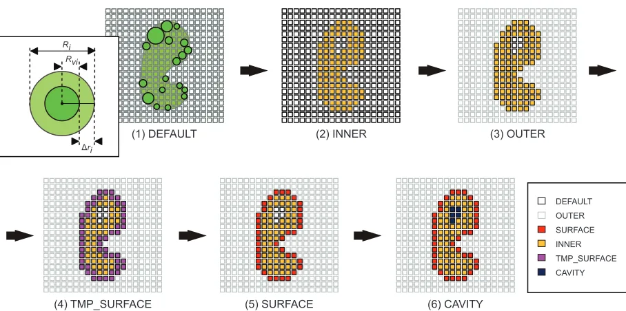
When the shape complementarity17–19_{between two proteins is} evaluated, the structure of a protein is converted into a rigid body object represented in a 3D grid space. Typically, in the protein–protein docking simulation, each point of the protein represented on the grid is classified as being in the core area, the surface area, or the cavity area as described below. Because the accuracy of docking simulations that use the shape complementarity search depends strongly on the representation method, various representation methods have been developed.

Here, we have developed a representation method called the voxel model, which has two distinguishing features. (1) The molecular surface can be faithfully modeled by changing the radius of the probe sphere to define as the extended solvent-accessible surface, which is traced out by the probe sphere center as it rolls over the protein, of each atomic type. (2) The shape complementarity can be determined much more accurately than just made voxel models by reducing the thickness of the molecular surface. However, when the thickness is reduced too much, the response of the shape complementarity evaluation function becomes too sensitive. Next we describe in detail the voxel model and the procedure for converting the crystal structure of a protein to the voxel model (voxelization).

Voxelization

The voxel model is expressed as shown in expression (1), where VOXEL (V) represents the voxel model, INNER (I) defines the area on the atom, where the protein exists, OUTER (O) is the area that is not INNER, in other words it indicates a solvent. SURFACE (S) is the area on the molecu-lar surface of the protein, CAVITY (C) is the area inside SURFACE that is not INNER, namely, it means a cavity. N is a set of natural numbers, and φ is an empty set. n_I, n_O, n_S, and n_C are the upper bound values of each voxel type (I, O, S, C) decided from the molecular size of the protein. All the areas in the voxel space in the initial state are defined as DEFAULT (D), and a temporary molecular surface of protein is defined as TMP_SURFACE (S_tmp).

(3)

Affinity evaluation and prediction system by using protein–protein docking

Dovepress

ν

= ∩ ∩ ∩ =

= ∈ ≤ ≤

=

{ , , , | }

{ | , }

{

I O S C I O S C

I I i i n

O O j j n

S

i I

j O

φ

N N

0 0

SS k k n

C C l l n

n n n n n n n

k S

I C

I O S C V V V

| , }

{ | , }

, , , | ,

∈ ≤ ≤

= ∈ ≤ ≤

≤ ≤ ∈ ≥

N N

N 0

0

0 0

00≤n_I +n_O +n_S+n_C ≤n n_V | _V ∈N,n_V ≥0 (1) The procedure of voxelization is formulated using expres-sion (2). Figure 1 details each step of this procedure.

ν

= → − → −

→ − →

( ) { } ( ) { , } ( )

{ , , } ( ) { , ,

step D step I D step

I O D step I O S

1 2 3

4 _ttmp D step

I O S D step I O S C

, } ( )

{ , , , } ( ) { , , , }

−

→ − →

5

6 ₍₂₎

• Step 1 (DEFAULT):

In the voxel space, all grid points are assigned to DEFAULT as the initial state.

• Step 2 (INNER):

The grid points that exist within a spheroid of radius R_i (=R_vi∆r_i) are assigned to INNER, where R_vi is the van der Waals radius of each atom, and ∆r_i is the increment in the radius of a defined type of atom.

• Step 3 (OUTER):

All the remaining grid points are assigned as OUTER.

• Step 4 (TMP_SURFACE):

The INNER grid points that adjoin the OUTER grid points are newly assigned to TMP_SURFACE.

• Step 5 (SURFACE):

A TMP_SURFACE grid point is finally replaced by SURFACE or INNER according to the following process. When a TMP_SURFACE grid point is enclosed by six or more OUTER grid points, the TMP_SURFACE grid point is re-assigned to SURFACE. After this process has been completed for all TMP_SURFACE grid points, the remain-ing TMP_SURFACE grid points are re-assigned to INNER. Thus, finally, the TMP_SURFACE grid points vanish from the voxel space.

• Step 6 (CAVITY):

The grid points which remain as DEFAULT are re-assigned to CAVITY. Hence, the DEFAULT grid points also disappear from the voxel space.

score function of contact surface area

In the shape complementarity evaluation, the surface contact between proteins represented by the grid points is evaluated by using the score function of the contact surface area.17 This score function defines a score for INNER, OUTER, SURFACE, and CAVITY as described in Voxelization. The contact surface score function we adopted for our voxel model is the pair-wise shape complementarity (PSC) score function S_PSC that Weng and colleagues17_{defined with ZDOCK.}17,18,20 As defined in expressions (3) and (4), this S_PSC is a primitive function where the electrostatic interaction is not considered. The score function S_PSC consists of two factors R_PSC, L_PSC.

DEFAULT OUTER SURFACE INNER TMP_SURFACE CAVITY

(1) DEFAULT (2) INNER (3) OUTER

(4) TMP_SURFACE (5) SURFACE (6) CAVITY

Rvi

Δ_ri

Ri

Figure six-step voxelization process for the quantization and characterization of protein surfaces in our AeP system.

Abbreviation: AeP, affinity evaluation and prediction.

(4)

Re[ ( , , )]

(

R l m n

number of SURFACE within OUTER vdw radius of Carb

PSC

= oon bonusR

otherwise

L l m n

SURFACE INNER o PSC +      = )

Re[ ( , , )]

, 0

1

0 ttherwise

R l m n L l m n

SURFACE INNER PSC PSC    = =

Im[ ( , , )] Im[ ( , , )] 3 9 ,,CAVITY OUTER 0      (3)

The factor R_PSC(l, m, n) is for the receptor protein, which is a protein fixed on the grid space, and the factor L_PSC(l, m, n) is for the probe protein, which is a protein that is rotated and translated on the grid space. In expressions (3) and (4), l, m, and n are the coordinates of the grid point, and “Re[]” and “Im[]”, respectively, indicate the real and imaginary parts of the factor and the PSC scoring function. Moreover, bonusR, which appears in the real part of R_PSC(l, m, n), indicates “bonus” points (ie, additional points added to the PSC scor-ing) when the probe protein penetrates the pocket structure of the receptor protein. The final S_PSC, as shown by expres-sion (4), is obtained by calculating the correlation function between R_PSC and L_PSC. The computational complexity of this calculation is O(N6_{), but can be decreased to O(N}3_{logN) by}

using a fast Fourier transform (FFT) as follows.

S o p q

R l m n L l o m p n q

PSC PSC PSC n N m N l N ( , , )

Re ( , , ) ( , , )

= ⋅ + + + = = =

∑

1 1 1       =  ⋅    −

Re ( ( ) ( ))

Im ( (

1

3

N IFT IFT R DFT L

N IFT IFT R

PSC PSC

P

PSC)⋅DFT L( PSC))

 



 (4)

Abbreviations: (DFT, Discrete Fourier Transform; IFT, Inverse Fourier transform).

In the S_PSC calculation, we adopted the FFT library CONV3D developed by Hourai and Nukada.16_{The CONV3D} is highly optimized for specific CPU architectures (Pentium, Xeon, Athlon, POWER5, etc.), achieves high-speed perfor-mance, and is about three times faster than the widely used FFT library package FFTW21,22_{(according to the results} obtained with Protein–Protein Docking Benchmark 2.0;23 data not shown).

At the beginning, a rotational search is performed in an actual evaluation of the contact surface between proteins. The rotational search works by explicitly rotating the ligand protein around each of its three Cartesian angles by a certain increment (15 degrees in this study). A total of 3600 rotated bodies of the ligand protein are thus generated. Next, the shape complementarity evaluation is undertaken for all rotated bodies. If the grid size of the ligand protein is N3_{, then} N3×_{3600 PSC scores must be calculated. Based on} prelimi-nary experiments, in all the analyses we only extracted the top-ranked 512 PSC scores for the following procedures.

Reliability of shape complementarity evaluation

To confirm the reliability of the shape complementarity evaluation by using our voxel model, we performed simple docking calculations using some bound structures adopted from Weng’s Protein–Protein Docking Benchmark 2.0 as samples. It is widely recognized that the main challenge in protein docking lies in the unbound–bound transition. Although we are also more interested in the unbound experi-ments than in the bound, the latter enables us to primitively confirm the advantages of our AEP’s improvement at the initial stage. Because a protein complex for the latter, which is pulled apart and reassembled, is more complementary than individually crystallized component structures for the former. The widely used i-RMSD (backbone RMSD at the interface) was the criterion we used to evaluate the reliability. In this way we evaluated the difference between the complex structure obtained by using the docking calculation and the X-ray crystal structure.

Affinity analysis

To calculate protein-protein affinity, we assess the biologi-cal relevance of target proteins by statistibiologi-cally analyzing the characteristics of shape complementarity. The affinity analysis involved processing the 512 top-ranked values of S_PSC obtained from the shape complementarity evaluation by using a clustering method that we call grouping. The follow-ing describes the affinity prediction procedure and includes a description of the grouping method.

• Step 1 (Shape complementarity evaluation):

A shape complementarity evaluation of protein pairs is performed. Only the 512 top-ranked S_PSC scores are then considered for step 2.

• Step 2 (Grouping):

The purpose of step 2 is to classify the 512 S_PSC scores into 10 clusters, C_i (i = 1–10). First, the clustering method is performed hierarchically by using the nearest neighbor

(5)

Dovepress

method for the 512 values of S_PSC as follows. We define the targeted dataset X = {x₁, ..., x₅₁₂} as consisting of 512 S_PSC scores from step 1. For each data point, x_i is represented as x_i= (S_i, T_i(T_X, T_Y, T_Z), R_i(R_, R_φ, R_ψ)). Here, S_i= S_PSC from expression (4), T_i(T_X, T_Y, T_Z) is the amount of translation for the ligand protein in the grid space, and R_i(R_, R_φ, R_ψ) is a rotation parameter for the ligand protein. If (o,p,q) in expression (4) is used, then o = T_X, p = T_Y, and q = T_Z in T_i(T_X, T_Y, T_Z), respectively.

All data x belonging to the dataset X are sorted by the rank order of S_i. In X, we define the data point with the maxi-mum S_i (maxS_i) as the central data y₁ of cluster 1 (y₁∈ C₁). Here, the term central data indicates data that represent a characteristic of a cluster. Now, we introduce the distances D₁(y₁, x_i) and D₂(y₁, x_i) between y₁ and x. Here, in this dataset x, the data y₁ is not included and is not classified into any clusters C_i (x_i∈ (C_i)C_{). The distance D}

1 is represented as the Euclidean translation distance, and the rotational distance D₂ is a value defined to represent the difference in rotation of data x_i and data y₁. Here, we define the center of gravity of a ligand as point G and the coordinates of the C_α atom in the C- and N-terminals of a ligand as points C and N, respectively. We also define vector u as the normal vector of a plane, which is defined by three points (G, C, and N). Thus, the rotational difference D₂ indicates the cosine between u_i of data x_i and u₁ of data y₁. When the following two conditions exist between the above data x_i (ie, x_i∈ (C_i)C_{) and the central data y}

1, the data x_i are classified into cluster 1 (C₁).

(1) When the translation distance |D₁| between T_i of data x_i and T₁ of the central data y₁ is less than a certain translational threshold (eg, 10.0Å).

(2) When the rotational distance |D₂| between x_i and y₁ is less than a certain rotational threshold (eg, π/6).

Cluster C₁ is determined by repeating step 2 for all x_i where y₁ is excluded. Similarly, step 2 is repeated for clusters C_i (i = 2–10). Step 2 ends either when the ten clusters (C₁–C₁₀) are generated or when all x_i belong to any cluster C_i.

• Step 3 (Calculation of Z-score):

The purpose of step 3 is to prepare for the affinity analysis. The Z-score indicates the number of standard deviations that an observation is above or below the mean. It allows us to compare observations from different normal distributions. Here, a set of central data y_i of each cluster C_i obtained in step 2 is defined as the central dataset Y. The distribution Z_score(y_i) is the Z-score distribution of the PSC score of each set of central data y_i∈ Y when the dataset X is considered a population. The distribution Z_conformation(C_i) is the distribu-tion of the Z-score of m_Ci. Here m_Ci is the number of data that

constitute cluster C_i when the dataset M_cluster= {m_ci | i ∈ N,

i  0} is considered a population. In step 3, the distributions

Z_score(y_i) and Z_conformation(C_i) are calculated.

• Step 4 (Calculation of affinity score S_affinity):

The measure for the affinity analysis is called an affinity score S_affinity, which is defined in expression (5) as the maximum value of a linear combination of Z_score(y_i) and Z_conformation(C_i) and their corresponding weighting factors w_s and w_c. The weighting factors w_s and w_c are introduced to determine the balance between the S_PSC score distribution Z_score(y_i) and the conformation distribution Z_conformation(C_i) when the affinity score S_affinity is calculated. The analysis of the affinity between protein pairs can be quantified by using S_affinity.

S w Z y w Z C

w weight

affinity s score i C conformation i

s

=max( ⋅ ( )+ ⋅ ( ))

: iing factor for y w weighting factor for Z

score i

e conformation

Z ( )

: (cc_i)

(5)

• Step 5:

Steps 1 to 4 are repeated. For example, if the affinity analysis is needed for 20 receptors and 20 ligands (20 × 20), then steps 1 to 4 are repeated 20 times because there are 20 ligands for each receptor. The S_affinity matrix is obtained by repeating steps 1–5 for all protein pairs.

When several target proteins have an unknown affinity, we can consider our AEP system to be an affinity prediction system. To evaluate the prediction performance of our AEP system, we used receiver operating characteristics curve (ROC) analysis. Based on the ROC analysis, we evaluated the maximum prediction performance of our AEP system by using a recall, a precision and a cutoff value. The parameters of w_s and w_c in expression (5) were defined at the maximum prediction performance.

Performance measures

Sensitivity and specificity are one of the performance measures for assessing the statistical significance of AEP’s predictions. The sensitivity or the recall measures the per-centage of biologically relevant pairs which are correctly identified as having the high-affinity scores; and the speci-ficity measures the percentage of biologically not relevant combinations which are identified as having the low-affinity. Here, the evaluation of each affinity scores (ie, high or low) is determined by a cutoff value from ROC analysis. Then, precision is the number of predictions statistically identi-fied as belonging to the protein pairs divided by the total number of pairs. “Accuracy” is closely related to precision, measures the percentage of correctly identified protein pairs

(6)

in the total number of pairs. Moreover, prevalence is defined as the total number of biologically relevant pairs in all the pairs. F-measure, which is the weighted harmonic mean of precision and recall, can be used as a single measure of performance.

implementation

Our AEP system was implemented using C language, which we ran on the cluster PC (16 cores and 64 GB memory). To improve the performance, we parallelized the core program of AEP using the Message-Passing Interface (MPI) library. For example, the time needed for the docking calculation is about 12 seconds for a grid size of 1283_{with a rotation} resolution of 15 degrees. Thus, the peak performance of AEP is 7,200 protein–protein pairs per day.

Protein pair dataset

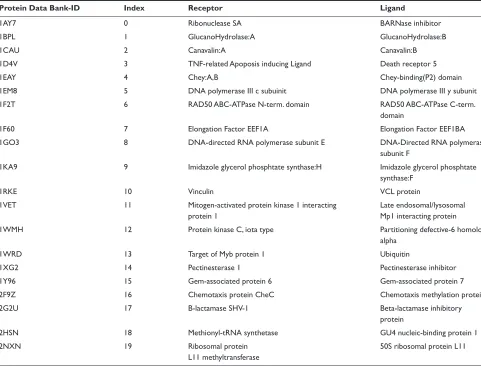
All protein pairs used in this study were selected manually from complex structures registered with the Protein Data

Bank (PDB). We adopted the 20 protein pairs (bound dataset) shown in Table 1, and analyzed the affinity of each pair.

In a docking simulation that uses a general shape comple-mentarity search, the receptor is fixed to the grid space and the ligand is rotated and translated in the grid space.

Results and discussion

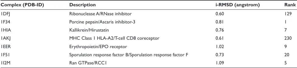
Validation of docking accuracy

using our AeP system

We selected seven protein pairs from Protein–Protein Docking Benchmark 2.0 according to the distribution of difficulty (“moderate”, “medium”, and “difficult”) that Weng and colleagues defined. The breakdown of the difficulty in the seven selected pairs was five pairs in the moderate difficultly class (1DFJ24_{, 1F34}25_{, 1HIA}26_{, 1AKJ}27_{, 1F51}28_{), one pair} (1I2M29_{) in the medium difficultly class and one pair (1EER}30₎ in the difficult class. Table 2 summarizes the docking calcu-lation results for seven protein pairs in which i-RMSD was

Table Targeted 20 protein pairs

Protein Data Bank-ID Index Receptor Ligand

1AY7 0 Ribonuclease sA BARnase inhibitor

1BPL 1 glucanohydrolase:A glucanohydrolase:B

1CAU 2 Canavalin:A Canavalin:B

1D4V 3 TnF-related Apoposis inducing Ligand Death receptor 5

1eAY 4 Chey:A,B Chey-binding(P2) domain

1eM8 5 DnA polymerase iii c subuinit DnA polymerase iii y subunit

1F2T 6 RAD50 ABC-ATPase n-term. domain RAD50 ABC-ATPase C-term.

domain

1F60 7 elongation Factor eeF1A elongation Factor eeF1BA

1gO3 8 DnA-directed RnA polymerase subunit e DnA-Directed RnA polymerase

subunit F

1KA9 9 imidazole glycerol phosphtate synthase:h imidazole glycerol phosphtate

synthase:F

1RKe 10 Vinculin VCL protein

1VeT 11 Mitogen-activated protein kinase 1 interacting

protein 1

Late endosomal/lysosomal Mp1 interacting protein

1WMh 12 Protein kinase C, iota type Partitioning defective-6 homolog

alpha

1WRD 13 Target of Myb protein 1 Ubiquitin

1Xg2 14 Pectinesterase 1 Pectinesterase inhibitor

1Y96 15 gem-associated protein 6 gem-associated protein 7

2F9Z 16 Chemotaxis protein CheC Chemotaxis methylation protein

2g2U 17 B-lactamase shV-1 Beta-lactamase inhibitory

protein

2hsn 18 Methionyl-tRnA synthetase gU4 nucleic-binding protein 1

2nXn 19 Ribosomal protein

L11 methyltransferase

50s ribosomal protein L11

(7)

Dovepress

used to confirm the reliability of the shape complementarity evaluation. For all seven pairs, i-RMSD  1.10 Å, indicating enough accuracy for docking prediction. As regards 1F34, 1HIA, 1EER, 1I2M, and 1F51, the rank that gives these highly accurate results is within the top 20 ranks. On the other hand, the S_PSC for 1DFJ and 1AKJ is relatively low, and therefore their ranks are also low, namely 129th and 230th, respectively. However, the affinity analysis successfully predicted the active sites of these pairs, including 1DFJ and 1AKJ. Although a general docking simulation uses a more complex evaluation function, the results obtained here by using a primitive evaluation function consisting only of the shape complementarity were good. Based on these docking results (Table 2), the shape complementarity evaluation is sufficiently reliable for affinity analysis.

shape complementarity evaluation

Prediction performance comparison between AeP and ZDOCK 3.0.1

As mentioned in Evaluation of shape complementarity, an original docking simulation code is included in our AEP system. We evaluated the prediction performance of the system when replacing our code with ZDOCK 3.0.1,31 which is a widely used docking program, and compared the prediction accuracy of the ZDOCK 3.0.1 version with that of the original AEP. It is the purpose of the comparison to show the effect of voxelization, grouping, and parallelization, which we have introduced.

We have already confirmed this effect. For this compari-son, we adopted 20 different protein pairs (bound dataset) from the Protein–Protein Docking Benchmark 2.0. The high-est score of ZDOCK 3.0.1 output was adopted as the affinity score for each protein pair.

The prediction performance obtained using ZDOCK 3.0.1 is shown in Table 3. This table represents the advantages of performance parameters of AEP over ZDOCK 3.0.1. Here, these parameters are of the peak performance by using the

chosen cutoff from the ROC analysis. The F-measure of AEP is 5.1% more accurate than that of ZDOCK 3.0.1. That means the high specificity of AEP over ZDOCK 3.0.1 while the difference of sensitivity is slightly 10.0% (ie, the difference of the value of true positives is only 2). AEP has an ability to correctly identify many true negatives (ie, TN = 307) with few false positives (ie, FP = 73) rather than ZDOCK 3.0.1 (ie, TN = 260, FP = 120). The ability to eliminate false positives is very important in terms of our goal that tries to deeply penetrate protein–protein networks. It is significantly valuable not to predict nonbonding pairs as well as identify-ing correct combinations.

Moreover, our AEP required much less computational time than ZDOCK 3.0.1. ZDOCK 3.0.1 needs over 3600 seconds for one protein pair whereas our AEP system needs only 12 seconds, namely it is 300 times faster. As shown by these results, we have revealed the advantage of our AEP with respect to prediction and computational performance.

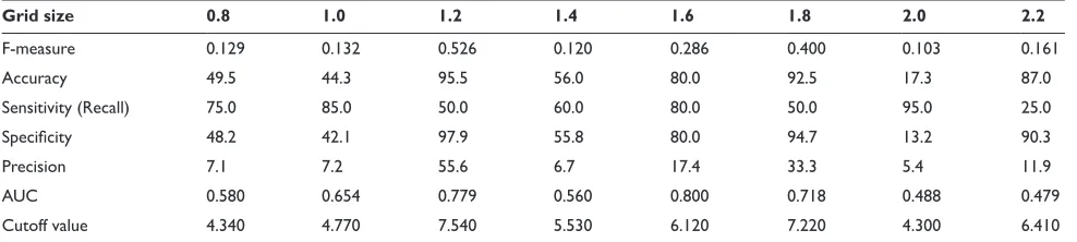
The effect of grid size

on the identification capability

of our affinity analysis

The accuracy of the representation of the protein model is dominated by the grid-size of the voxelization procedure. In shape complementarity docking, the optimum grid size is defined as being 1.2 Å by Weng and colleagues17_{as regards} accuracy of docking, although, for our affinity analysis, which is derived from that shape complementarity docking scheme, the optimum grid size is unclear. Thus, we first investigated an optimal grid size for our affinity analysis. In this investigation using 20 × 20 protein pairs as shown in Table 1, the grid size ranged from 0.8 to 2.2 Å at 0.2 Å intervals. As the standard for our evaluation of the accuracy of the affinity analysis we used F-measure, which we obtained as the cutoff value from the ROC analysis. The results of F-measure are shown in Table 4.

Table Docking calculation results to validate the shape complementarity evaluation using voxel model

Complex (PDB-ID) Description i-RMSD (angstrom) Rank

1DFJ Ribonuclease A/Rnase inhibitor 0.60 129

1F34 Porcine pepsin/Ascaris inhibitor-3 0.81 1

1hiA Kallikrein/hirustatin 0.76 7

1AKJ MhC Class 1 hLA-A2/T-cell CD8 coreceptor 0.61 230

1eeR erythropoietin/ePO receptor 1.02 9

1F51 sporulation response factor B/sporulation response factor F 0.73 20

1i2M Ran gTPase/RCC1 1.09 5

Abbreviations: i-RMsD, backbone root mean square at the interface; PDB-iD, Protein Data Bank-iD.

(8)

According to these results, the highest F-measure was derived with a grid size of 1.2 Å. Thus, we use this grid size for all analyses as mentioned below.

evaluation for 20 × 20 protein pairs

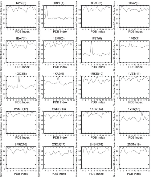
Figure 2 shows the results of the shape complementarity evaluation for about 20 × 20 protein pairs. It also shows the normalized S_PSC for the receptor of each ligand. The vertical axis shows the normalized S_PSC where the maximum value is 1.0, and the horizontal axis shows the PDB index of the receptors (The relation between the index and PDB-ID is shown in Table 1).

The polygonal lines of 12 out of 20 receptors have no characteristic peak. For these receptors, the score of each predicted ligand is not the maximum (ie, S_PSC  1.0) or the number of ligands with maximal score is not only one: 1AY732_(index= _{0), 1CAU}33_{(2), 1D4V}34_{(3), 1EAY}35_(4), 1EM836_{(5), 1VET}37_{(11), 1WMH}38_{(12), 1WRD}39_(13), 1XG240_{(14), 2F9Z}41_{(16), 2HSN}42_{(18), and 2NXN}43_(19). Thus, when using only the normalized S_PSC, it is too dif-ficult to evaluate and quantify the affinity between ligand and receptor.

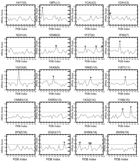
Using our affinity calculation, Figures 3 and 4 show the affinity score S_affinity with w_c= 0 and w_s= 1. These values for

w_c and w_s (parameters used for calculating affinity scores) were chosen to provide the maximum prediction performance (ie, F-measure) from our preliminary experiments.

Figure 3 shows the S_affinity of the receptor of each ligand, and the vertical axis shows the S_affinity and the horizontal axis shows the PDB index of the receptor. When our AEP system is used as a prediction system, the horizontal dotted line shows that the cutoff value at which the system achieves its maximum prediction performance is 7.54σ. This value pro-vides the optimal tradeoff between sensitivity and specific-ity. Each filled arrowhead () denotes a protein pair where S_affinity exceeds the chosen cutoff value, thus indicating that the biologically relevant pair with a statistically significant score; each unfilled arrowhead is a protein pair incorrectly identified as being biologically relevant (ie, false positive).

Figure 4 shows the S_affinity matrix in which the 10 data points (denoted by circles) along the diagonal of the matrix represent the protein pairs that have been experimentally confirmed to be biologically relevant. The vertical axis shows the index of the ligand, and the horizontal axis that of the receptor.

Based on Figures 2 and 3, the S_affinity obtained by our grouping process is more suitable than the simple S_PSC for estimating protein–protein affinity. For example, the S_affinity for a specific ligand is the highest for the following receptors: 1BPL44_{(1), 1F60}45_{(7), 1GO3}46_{(8), 1KA9}47_{(9), 1RKE}48_(10), 1VET(11), 1Y9649_{(15), 2G2U}50_{(17), and 2NXN(19). These} protein pairs with the highest score are also biologically relevant pairs. Moreover, for 1F2T51_{(6), the S}

affinity of a

bio-logically relevant pair is the 2nd high score.

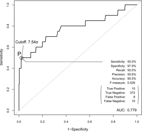
Our AEP system can therefore constitute a prediction system if we introduce a recall, a precision and a cutoff value. Our system predicts pairs whose S_affinity exceeds the cutoff value and are thus biologically relevant pairs. Based on the ROC curve in Figure 5, a cutoff value of 7.54σ dem-onstrates the maximal prediction performance of our system.

Table Comparison prediction performance between AeP and

ZDOCK

Parameters ZDOCK

(grid size = .)

AEP

(grid size = .)

F-measure 0.194 0.245

Accuracy 68.8 80.0

sensitivity (Recall) 75.0 65.0

Specificity 68.4 80.8

Precision 11.1 15.1

AUC 0.776 0.744

Abbreviation: AEP, affinity evaluation and prediction; AUC, area under the curve.

Table evaluations about the prediction performance for various of grid size

Grid size 0. .0 . . . . .0 .

F-measure 0.129 0.132 0.526 0.120 0.286 0.400 0.103 0.161

Accuracy 49.5 44.3 95.5 56.0 80.0 92.5 17.3 87.0

sensitivity (Recall) 75.0 85.0 50.0 60.0 80.0 50.0 95.0 25.0

Specificity 48.2 42.1 97.9 55.8 80.0 94.7 13.2 90.3

Precision 7.1 7.2 55.6 6.7 17.4 33.3 5.4 11.9

AUC 0.580 0.654 0.779 0.560 0.800 0.718 0.488 0.479

Cutoff value 4.340 4.770 7.540 5.530 6.120 7.220 4.300 6.410

Abbreviation: AUC, area under the curve.

(9)

Affinity evaluation and prediction system by using protein–protein docking Dovepress 0 0.2 0.4 0.6 0.8 1

0 2 4 6 8 10 12 14 16 18 20

Normalized Contact Surface Score PDB Index

1AY7(0) 0 0.2 0.4 0.6 0.8 1 0 0.2 0.4 0.6 0.8 1 0 0.2 0.4 0.6 0.8 1 0 0.2 0.4 0.6 0.8 1 0 0.2 0.4 0.6 0.8 1 0 0.2 0.4 0.6 0.8 1 0 2 4 6 8 10 12 14 16 18 20

1BPL(1)

0 2 4 6 8 10 12 14 16 18 20

1CAU(2) 0 0.2 0.4 0.6 0.8 1

0 2 4 6 8 10 12 14 16 18 20

1D4V(3) 0 0.2 0.4 0.6 0.8 1

0 2 4 6 8 10 12 14 16 18 20

1EAY(4) 0 0.2 0.4 0.6 0.8 1

0 2 4 6 8 10 12 14 16 18 20

1EM8(5)

0 2 4 6 8 10 12 14 16 18 20

1F2T(6) 0 0.2 0.4 0.6 0.8 1

0 2 4 6 8 10 12 14 16 18 20

1F60(7) 0 0.2 0.4 0.6 0.8 1 0 0.2 0.4 0.6 0.8 1 0 0.2 0.4 0.6 0.8 1

0 2 4 6 8 10 12 14 16 18 20

1GO3(8) 0 0.2 0.4 0.6 0.8 1

0 2 4 6 8 10 12 14 16 18 20

1KA9(9)

0 2 4 6 8 10 12 14 16 18 20

1RKE(10) 0 0.2 0.4 0.6 0.8 1

0 2 4 6 8 10 12 14 16 18 20

1VET(11)

0 2 4 6 8 10 12 14 16 18 20

1WMH(12) 0 0.2 0.4 0.6 0.8 1

0 2 4 6 8 10 12 14 16 18 20

1WRD(13)

0 2 4 6 8 10 12 14 16 18 20

1XG2(14) 0 0.2 0.4 0.6 0.8 1

0 2 4 6 8 10 12 14 16 18 20

1Y96(15)

0 2 4 6 8 10 12 14 16 18 20

2F9Z(16) 0 0.2 0.4 0.6 0.8 1

0 2 4 6 8 10 12 14 16 18 20

2G2U(17)

0 2 4 6 8 10 12 14 16 18 20

2HSN(18) 0 0.2 0.4 0.6 0.8 1

0 2 4 6 8 10 12 14 16 18 20

2NXN(19)

Figure normalized PsC score SSPC of the receptor of each ligand. The horizontal axis shows the PDB index as in Table 1, and the vertical axis shows the normalized PsC

score SSPC.

Abbreviations: PDB,Protein Data Bank; PsC, pair-wise shape complementarity.

(10)

When this cutoff is adopted, the performance of our AEP as a prediction system has an F-measure of 0.526, a recall of 50.0%, a precision of 55.6% (sensitivity of 50.0% and a specificity of 97.9%), and an accuracy of 95.5%. When we consider that the prevalence of the current sample size is

5%, this performance is sufficiently high. Our AEP system identified 10 of 20 biologically relevant combinations from among 400 pairs of combination candidates. In addition, because our AEP system can identify the true negative pairs, the specificity and the accuracy are sufficiently high at 97.9%,

2 4 6 8 10 12

0 2 4 6 8 10 12 14 16 18 20

Affinity Score PDB Index 1AY7(0) 2 4 6 8 10 12

0 2 4 6 8 10 12 14 16 18 20

Affinity Score PDB Index 1BPL(1) 2 4 6 8 10 12

0 2 4 6 8 10 12 14 16 18 20

Affinity Score PDB Index 1CAU(2) 2 4 6 8 10 12

0 2 4 6 8 10 12 14 16 18 20

Affinity Score PDB Index 1D4V(3) 2 4 6 8 10 12

0 2 4 6 8 10 12 14 16 18 20

Affinity Score PDB Index 1EAY(4) 2 4 6 8 10 12

0 2 4 6 8 10 12 14 16 18 20

Affinity Score PDB Index 1EM8(5) 2 4 6 8 10 12

0 2 4 6 8 10 12 14 16 18 20

Affinity Score PDB Index 1F2T(6) 2 4 6 8 10 12

0 2 4 6 8 10 12 14 16 18 20

Affinity Score PDB Index 1F60(7) 2 4 6 8 10 12

0 2 4 6 8 10 12 14 16 18 20

Affinity Score PDB Index 1GO3(8) 2 4 6 8 10 12

0 2 4 6 8 10 12 14 16 18 20

Affinity Score PDB Index 1KA9(9) 2 4 6 8 10 12

0 2 4 6 8 10 12 14 16 18 20

Affinity Score PDB Index 1RKE(10) 2 4 6 8 10 12

0 2 4 6 8 10 12 14 16 18 20

Affinity Score PDB Index 1VET(11) 2 4 6 8 10 12

0 2 4 6 8 10 12 14 16 18 20

Affinity Score PDB Index 1WMH(12) 2 4 6 8 10 12

0 2 4 6 8 10 12 14 16 18 20

Affinity Score PDB Index 1WRD(13) 2 4 6 8 10 12

0 2 4 6 8 10 12 14 16 18 20

Affinity Score PDB Index 1XG2(14) 2 4 6 8 10 12

0 2 4 6 8 10 12 14 16 18 20

Affinity Score PDB Index 1Y96(15) 2 4 6 8 10 12

0 2 4 6 8 10 12 14 16 18 20

Affinity Score PDB Index 2F9Z(16) 2 4 6 8 10 12

0 2 4 6 8 10 12 14 16 18 20

Affinity Score PDB Index 2G2U(17) 2 4 6 8 10 12

0 2 4 6 8 10 12 14 16 18 20

Affinity Score PDB Index 2HSN(18) 2 4 6 8 10 12

0 2 4 6 8 10 12 14 16 18 20

Affinity Score

PDB Index 2NXN(19)

Figure Affinity score Saffinity of the receptor of each ligand. The cutoff value is 7.54σ. The filled arrowhead () denotes a protein pair in which Saffinity 7.54σ and is thus

biologically relevant; the unfilled arrowhead is a protein pair incorrectly identified as being biologically relevant (ie, false positive). The horizontal axis shows the PDB index, and the vertical axis shows the affinity score Saffinity.

Abbreviation: PDB, Protein Data Bank.

(11)

Dovepress

95.5%, respectively. This means that the prediction provided by our AEP system is reliable.

Efficacy of “asymmetrically biased” PSC

score function for affinity analysis results

by comparison of molecular size

We compiled the relationship between the number of atoms in terms of a molecular size and the results of the affinity analysis as shown in Figure 6. There is a relation between the affinity results and the size of receptors or ligands. This size indicates the number of atoms for a protein. The cor-relation coefficient between the identification probability of biologically relevant pairs and the size of receptor is 0.40. This positive correlation is related to the characteristic of the score function of the shape complementarity. As mentioned above, the score function we used for the receptor is differ-ent from that for the ligand. Because the score function for a receptor has a “bias” that tends to pull into the ligand to

own pocket structure, we expect our AEP system to exhibit increasing docking structure accuracy when searching between a “large” receptor and a “small” ligand. The cur-rent results reveal the efficacy as regards the evaluation of affinity. Moreover, because this characteristic is always good for a molecule that consists of a large number of atoms, to make the estimation performance more accurate, the dataset should be rearranged in terms of the assignment of either a receptor or a ligand by the order of the molecular size. In other word, a “large” molecule should always be assigned as a receptor regardless of whether it functions biologically as a receptor or a ligand.

Problem with shape complementarity

evaluation

In the current affinity analysis, our AEP system succeeded in predicting the following 10 biologically relevant protein pairs from 400 (ie, 20 × 20) protein pairs: 1BPL(1), 1F2T(6),

Saffinity Receptor

Li

ga

nd

0

10

5

1

2

3

4

6

7

8

9

15

11

12

13

14

16

17

18

19

(index)

0 1 2 3 4 5 6 7 8 9 10 11 12 13 14 15 16 17 18 19 (index)

0.0 7.0

Figure Matrix of affinity score Saffinity with weighting parameters wc= 0, and ws= 1. The points on the diagonal line show the biologically relevant pairs, and the circles show

the biologically relevant pairs where the AeP system provided a successful prediction.

Abbreviation: AEP, affinity evaluation and prediction.

(12)

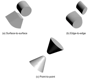
1F60(7), 1GO3(8), 1KA9(9), 1RKE(10), 1VET(11), 1Y69(15), 2G2U(17), and 2NXN(19). The common feature of those complex structures is that, except for 1F2T(6) and 1Y96(15), they have a typical docking type that we called “surface-to-surface”. The ”surface-to-surface” type as shown in Figure 7(a) is docking formed under a wide contact sur-face. Even the affinity evaluation was derived from a shape complementarity search, because in practice, the affinity analysis revealed that a shape complementarity search can identify a pair with such a docking type in a sophisticated manner from 400 protein pair candidates.

In addition, the docking type of 1F2T(6) or 1Y96(15) is different from the typical type as mentioned above. We call

their docking type “edge-to-edge”. The “edge-to-edge” type is a docking style where the edge of the surface of a receptor comes in contact with a ligand edge as shown in Figure 7(b). Naturally, a shape complementarity search has difficulty in dealing with the “edge-to-edge” docking type. Indeed as shown in Figure 3, with 1F2T(6), even our AEP system suc-ceeded in predicting the pair, and the affinity score from the correct pair is the 2nd highest score rather than the highest. Our AEP system also succeeded for 1Y96(15), however, the 2nd highest score from an irrelevant pair is also over the cutoff value of 7.54σ.

On the other hand, our AEP system failed to predict the following 10 biologically relevant pairs: 1AY7(0), 1CAU(2),

0.0 0.2 0.4 0.6 0.8 1.0

0.0

0.2

0.4

0.6

0.8

1.0

1−Specificity

Sensitivity

Cutoff: 7.54σ

P

AUC: 0.779

Sensitivity: Specificity:

Precision: Recall:

Accuracy: F-measure:

(

True Positive:

True Negative: False Positive: False Negative:

50.0% 97.9% 50.0% 55.6% 95.5% 0.526

10

372

8 10

)

Figure The ROC curve for the prediction performance of the AeP system. The peak performance achieved at point P (cutoff value is 7.54σ), and their values are shown in the bottom-right corner.

Abbreviations: AEP, affinity evaluation and prediction; ROC, receiver operating characteristics.

(13)

Dovepress

1AY7(0) _1BPL(1)

1D4V(3) 1F2T(6)

1F60(7)

1CAU(2) 1EM8(5)

1GO3(8)

1KA9(9) 1RKE(10)

1VET(11) 1WMH(12)1WRD(13)

1XG2(14)

1Y96(15)

2F9Z(16)

2G2U(17)

2HSN(18)

2NXN(19)1EAY(4)

0 1000 2000 3000 4000 5000

0 1000 2000 3000 4000

No. of Atoms in Receptor Protein

N

o.

o

f A

to

m

s

in

L

ig

an

d

Pr

ot

ei

n

3500 2500

1500 500

Figure Relation between the size of each protein pair (ie, number of atoms) needed for biological relevance and the affinity analysis results. The horizontal axis shows the number of atoms in the receptor, and the vertical axis shows that in the ligand. The symbols denote the protein pair. The unfilled circles () denote a protein pair that was identified as biologically relevant by the AEP system, and the filled circles () denotes a protein pair identified as not biologically relevant.

Abbreviation: AEP, affinity evaluation and prediction.

(a) Surface-to-surface (b) Edge-to-edge

(c) Point-to-point

Figure Models for docking styles. Type (a), called “surface-to-surface”, is most popular docking among our docking complex structures. Type (b) is called “edged-to-edge” contacting only using each edge of receptor and ligand. Type (c) is called “point-to-point” which is most less performance by shape complementarity search.

(14)

1D4V(3), 1EAY(4), 1EM8(5), 1WHM(12), 1WRD(13), 1XG2(14), 2F9Z(16), and 2HSN(18). This prediction failure might be due to a structural feature of the protein pair that hinders the shape complementarity evaluation.

Because the docking type of 1AY7(0), 1CAU(2), 1EAY(4), 1WHM(12), 1WRD(13), 1XG2(14), and 2F9Z(16) is “edge-to-edge”, the affinity scores S_affinity are low (ie, under 7.54σ) for almost all the ligands. The complex structures of 1D4V(3), 1EM8(5), and 2HSN(18) are “point-to-point” docking type. This docking type has a smaller contact surface area than the “edge-to-edge” type as shown in Figure 7(c). In fact, the docking site of the 1EM8(5) receptor is too small to allow us to detect the correct pair. This makes a shape complementarity search difficult to perform with this type.

Most of the protein pairs that our AEP system failed to predict were not the typical docking type (ie, surface-to-surface) with a complex formation as mentioned above but edge-to-edge and/or point-to-point type, because the shape complementarity search cannot deal easily with these types. We are now extract-ing the common characteristics from these negative dockextract-ing types and developing methods to overcome these issues.

Conclusion

A shape complementarity search method and a statistical method called ‘grouping’ were combined to evaluate and predict the affinity between various protein pairs with known structures. At a prevalence of 5.0%, prediction with our AEP system had a recall of 50.0%, a precision of 55.6% and an accuracy of 95.5%. An evaluation of the affinity was difficult when only the PSC score based on the shape complementarity evaluation was considered.

The affinity evaluation was significantly improved by the grouping process that we introduced. Future research will be undertaken on the relation between the physicochemical characteristic of proteins and the prediction accuracy of our AEP system, and then, based on those findings, research will be undertaken on further improving the accuracy of the sys-tem. Although an unbound dataset was not considered in this study, our future research will also include how to improve the prediction accuracy of an unbound dataset.

Disclosure

The authors report no conflicts of interest in this work.

References

1. Jones S, Thornton JM. Principles of protein-protein interactions. Proc Natl Acad Sci U S A. 1996;93:13–20.

2. Teichmann SA. Principles of protein-protein interactions. Bioinformatics. 2002;18:S249–S249.

3. Ayub MJ, Smulski CR, Nyambega B, et al. Protein-protein interaction map of the Trypanosoma cruzi ribosomal P protein complex. Gene. 2005;357:129–136.

4. Rual JF, Venkatesan K, Hao T, et al. Towards a proteome-scale map of the human protein-protein interaction network. Nature. 2005;437:1173–1178.

5. Collins SR, Miller KM, Maas NL, et al. Functional dissection of pro-tein complexes involved in yeast chromosome biology using a genetic interaction map. Nature. 2007;446:806–810.

6. Parrish JR, Yu JK, Liu GZ, et al. A proteome-wide protein interaction map for Campylobacter jejuni. Genome Biol. 2007;8:R130.

7. Wong J, Nakajima Y, Westermann S, et al. A protein interaction map of the mitotic spindle. Mol Biol Cell. 2007;18:3800–3809.

8. Giot L, Bader JS, Brouwer C, et al. A protein interaction map of Drosophila melanogaster. Science. 2003;302:1727–1736.

9. Stanyon CA, Liu GZ, Mangiola BA, et al. A Drosophila protein-interaction map centered on cell-cycle regulators. Genome Biol. 2004;5:R96. 10. Rain JC, Selig L, De Reuse H, et al. The protein-protein interaction

map of Helicobacter pylori. Nature. 2001;409:211–215.

11. Wojcik J, Schachter V. Protein-protein interaction map inference using interacting domain profile pairs. Bioinformatics. 2001;17(Suppl 1): S296–S305.

12. Ofran Y, Rost B. Predicted protein-protein interaction sites from local sequence information. FEBS Lett. 2003;544:236–239.

13. Smith GR, Sternberg MJ. Prediction of protein-protein interactions by docking methods. Curr Opin Struct Biol. 2002;12:28–35.

14. Park DU, Lee SM, Bolser D, et al. Comparative interactomics analysis of protein family interaction networks using PSIMAP (protein structural interactome map). Bioinformatics. 2005;21:3234–3240.

15. Gong S, Yoon G, Jang I, et al. PSIbase: A database of Protein Structural Interactome map (PSIMAP). Bioinformatics. 2005;21:2541–2543. 16. Nukada A, Hourai Y, Nishida A. High performance 3D convolution for

protein docking on IBM Blue Gene. Proc. ISPA2007, Lecture Notes in Computer Science. 2007;4742:958–969.

17. Chen R, Li L, Weng ZP. ZDOCK: An initial-stage protein-docking algorithm. Proteins. 2003;52:80–87.

18. Chen R, Tong WW, Mintseris J, Li L, Weng ZP. ZDOCK predictions for the CAPRI Challenge. Proteins. 2003;52:68–73.

19. Pierce B, Tong WW, Weng ZP. M-ZDOCK: a grid-based approach for C-n symmetric multimer docking. Bioinformatics. 2005;21: 1472–1478.

20. Zhang C, Liu S, Zhou YQ. Docking prediction using biological informa-tion, ZDOCK sampling technique, and clustering guided by the DFIRE statistical energy function. Proteins. 2005;60:314–318.

21. Kiselyov O, Taha W. Relating FFTW and split-radix. Embedded Soft-ware and Systems. 2005;3605:488–493.

22. Vuduc R, Demmel JW. Code generators for automatic tuning of numerical kernels: Experiences with FFTW - Position paper. Semantics, Applications and Implementation of Program Generation, Proceedings. 2000;1924:190–211.

23. Mintseris J, Wiehe K, Pierce B, et al. Protein-protein docking bench-mark 2.0: An update. Proteins. 2005;60:214–216.

24. Kobe B, Deisenhofer J. A structural basis of the interactions between leucine-rich repeats and protein ligands. Nature. 1995;374:183–186. 25. Ng KKS, Petersen JFW, Cherney MM, et al. Structural basis for the

inhibition of porcine pepsin by Ascaris pepsin inhibitor-3. Nature Struct Biol. 2000;7:653–657.

26. Mittl PRE, DiMarco S, Fendrich G, et al. A new structural class of serine protease inhibitors revealed by the structure of the hirustasin-kallikrein complex. Structure. 1997;5:585–585.

27. Gao GF, Tormo J, Gerth UC, et al. Crystal structure of the complex between human CD8 alpha alpha and HLA-A2. Nature. 1997;387: 630–634.

28. Zapf J, Sen U, Madhusudan, Hoch JA, Varughese KI. A transient inter-action between two phosphorelay proteins trapped in a crystal lattice reveals the mechanism of molecular recognition and phosphotransfer in signal transduction. Structure. 2000;8:851–862.

(15)

Advances and Applications in Bioinformatics and Chemistry

Publish your work in this journal

Submit your manuscript here: http://www.dovepress.com/advances-and-applications-in-bioinformatics-and-chemistry-journal

Advances and Applications in Bioinformatics and Chemistry is an international, peer-reviewed open-access journal that publishes articles in the following fields: Computational biomodelling; Bioinformatics; Computational genomics; Molecular modelling; Protein structure modelling and structural genomics; Systems Biology; Computational

Biochemistry; Computational Biophysics; Chemoinformatics and Drug Design; In silico ADME/Tox prediction. The manuscript management system is completely online and includes a very quick and fair peer-review system, which is all easy to use. Visit http://www.dovepress.com/ testimonials.php to read real quotes from published authors.

Dovepress

Dove

press

29. Renault L, Kuhlmann J, Henkel A, Wittinghofer A. Structural basis for guanine nucleotide exchange on Ran by the regulator of chromosome condensation (RCC1). Cell. 2001;105:245–255.

30. Syed RS, Reid SW, Li CW, et al. Efficiency of signalling through cytokine receptors depends critically on receptor orientation. Nature. 1998;395:511–516.

31. Mintseris J, Pierce B, Wiehe K, Anderson R, Chen R, Weng ZP. Integrating statistical pair potentials into protein complex prediction. Proteins. 2007;69:511–520.

32. Sevcik J, Urbanikova L, Dauter Z, Wilson KS. Recognition of RNase Sa by the Inhibitor Barstar: Structure of the complex at 1.7 angstrom resolution. Acta Crystallogr D Biol Crystallogr. 1998;54:954–963. 33. Ko TP, Ng JD, Day J, Greenwood A, Mcpherson A. Determination of

three crystal structures of canavalin by molecular replacement. Acta Crystallogr D Biol Crystallogr. 1993;49:478–489.

34. Mongkolsapaya J, Grimes JM, Chen N, et al. Structure of the TRAIL-DR5 complex reveals mechanisms conferring specificity in apoptotic initiation. Nature Struct Biol. 1999;6:1048–1053.

35. McEvoy MM, Hausrath AC, Randolph GB, Remington SJ, Dahlquist FW. Two binding modes reveal flexibility in kinase/response regulator interactions in the bacterial chemotaxis pathway. Proc Natl Acad Sci U S A. 1998;95:7333–7338.

36. Gulbis JM, Kazmirski SL, Finkelstein J, Kelman Z, O’Donnell M, Kuriyan J. Crystal structure of the chi: psi subassembly of the Escherichia coli DNA polymerase clamp-loader complex. Eur J Biochem. 2004;271:439–449.

37. Kurzbauer R, Teis D, de Araujo MEG, et al. Crystal structure of the p14/MP1 scaffolding complex flow a twin couple attaches mitogen-activated protein kinase signaling to late endosomes. Proc Natl Acad Sci U S A. 2004;101:10984–10989.

38. Hirano Y, Yoshinaga S, Takeya R, et al. Structure of a cell polarity regulator, a complex between atypical PKC and Par6 PB1 domains. J Biol Chem. 2005;280:9653–9661.

39. Akutsu M, Kawasaki M, Katoh Y, et al. Structural basis for recognition of ubiquitinated cargo by Tom1-GAT domain. Febs Lett. 10 2005;579:5385–5391.

40. Di Matteo A, Giovane A, Raiola A, et al. Structural basis for the inter-action between pectin methylesterase and a specific inhibitor protein. Plant Cell. 2005;17:849–858.

41. Chao XJ, Muff TJ, Park SY, et al. A receptor-modifying deamidase in complex with a signaling phosphatase reveals reciprocal regulation. Cell. 2006;124:561–571.

42. Simader H, Hothorn M, Kohler C, Basquin J, Simos G, Suck D. Structural basis of yeast aminoacyl-tRNA synthetase complex formation revealed by crystal structures of two binary sub-complexes. Nucleic Acid Res. 2006;34:3968–3979.

43. Demirci H, Gregory ST, Dahlberg AE, Jogl G. Recognition of ribosomal protein L11 by the protein trimethyltransferase PrmA. Embo J. 2007;26:567–577.

44. Machius M, Wiegand G, Huber R. Crystal-structure of calcium-depleted Bacillus-licheniformis alpha-amylase at 2.2-angstrom resolution. J Mol Biol. 1995;246:545–559.

45. Andersen GR, Pedersen L, Valente L, et al. Structural basis for nucleo-tide exchange and competition with tRNA in the yeast elongation factor complex eEF1A: eEF1B alpha. Mol Cell. 2000;6:1261–1266. 46. Todone F, Brick P, Werner F, Weinzierl ROJ, Onesti S. Structure of an

archaeal homolog of the eukaryotic RNA polymerase II RPB4/RPB7 complex. Mol Cell. 2001;8:1137–1143.

47. Omi R, Mizuguchi H, Goto M, et al. Structure of imidazole glyc-erol phosphate synthase from Thermus thermophilus HB8: Open-closed conformational change and ammonia tunneling. J Biochem. 2002;132:759–765.

48. Izard T, Evans G, Borgon RA, Rush CL, Bricogne G, Bois PRJ. Vinculin activation by talin through helical bundle conversion. Nature. 2004;427:171–175.

49. Ma YL, Dostie J, Dreyfuss G, Van Duyne GD. The Gemin6-Gemin7 heterodimer from the survival of motor neurons complex has an Sm protein-like structure. Structure. 2005;13:883–892.

50. Reynolds KA, Thomson JM, Corbett KD, et al. Structural and compu-tational characterization of the SHV-1 beta-lactamase-beta- lactamase inhibitor protein interface. J Biol Chem. 2006;281:26745–26753. 51. Hopfner KP, Karcher A, Shin DS, et al. Structural biology of Rad50

ATPase: ATP-driven conformational control in DNA double-strand break repair and the ABC-ATPase superfamily. Cell. 2000;101:789–800.