Volume 78 – No.14, September 2013
Association Rule Mining Algorithm’s Variant Analysis
Prince Verma
Assistant Professor CSE Dept. CT Institute of Engg., Mgt. & Tech.Punjab, India
Dinesh Kumar
Associate Professor IT Dept. DAV Institute of Eng. & Tech.Punjab, India
ABSTRACT
Association rule mining is a vital technique of data mining which is of great use and importance. For Association Rule mining various new techniques have been developed but concept for the newly developed algorithms remains the same. These recent developments are basically modifications to previous ones which introduce some minute changes in existing algorithms for better results. This paper addresses these basic algorithms and techniques in an elaborative way. So the reader can understand each of these techniques along with their pros and cons, without any additional effort. The techniques discussed here involve AIS, SETM, Apriori and FP-tree in detail.
Keywords
Data Mining, KDD Process, Association Rule Mining, Pruning.
1.
INTRODUCTION
Originally, “DATA MINING" is statistician's term which means the overuse of data to obtain valid inferences. So, it is the discovery of useful summaries of data. Data Mining is the process to discover the knowledge or hidden pattern from large databases [5]. It is a useful method required for the intersection of machine learning, dbase systems, AI (artificial intelligence) and statistics. It works on the principle of retrieving relevant information from data. It is mainly in use of financial analysts, banks, insurance companies, retail stores, business intelligence organizations, and hospitals, to extract the useful information that they require from large databases. The goal of this process is to create and find accurate patterns that are not previously known by us. So, the overall goal of data mining is to extract and obtain information from databases and transform it into an understandable format for use in future. In actual data mining task as in [5] can be automatic or semi-automatic to extract the unknown patterns.
1.1 Data Mining Tasks
Data mining may involve six classes of tasks in common:
Anomaly detection – It is identification of unusual data records that might have errors and are un-interesting. Association rule learning (Dependency modeling) – It is
the process of searching relationships between variables in provided database.
Clustering – It is the task of discovering groups and structures in the data that can be similar in some way or another, without using any known structures. Classification – It is the process of generalizing known
structure to apply to new data.
Regression – It attempts to find a function that create model of data with the minimum errors.
Summarization – It is process of creating a compact representation of the data set, including report generation and visualization.
1.2 Data Mining Process
Data Mining can also be seen as one of the core processes of Knowledge Discovery in Database (KDD).
It can be viewed as process of Knowledge Discovery in Databases [15]:
Data Extraction/gathering: To collect the data from sources. e.g., data warehousing, Web crawling. Data cleansing: To eliminate bogus data or/and errors,
e.g., atmospheric temperature = 150.
Feature extraction: To extract only task relevant data, i.e to obtain the interesting attributes of data,
Pattern extraction and discovery: This step is seen as process of “data mining”, where one should concentrate the effort.
[image:1.595.317.564.421.597.2]Visualization of the data and Evaluation of results: To create knowledge base.
Figure 1: KDD process [15]
The specific approaches, however, differ from one researcher to other and one company to the other. For example: IBM in [4, 15] defined four major operations for Data Mining:
Predictive modelling: that uses inductive reasoning techniques i.e. neural networks and inductive reasoning algorithms for creating predictive models. Database segmentation: that partition data into clusters
using statistical clustering techniques.
Link analysis: It involved identifying useful and meaningful associations in data.
Deviation detection: It detects and explains why certain records could not be inserted into specific segments. Databases
Data Warehouse
Data Mining
Visualization and Pattern Evaluation
Feature Extraction
Data Extraction and Cleaning
Patterns
Task Relevant / Processed Data
Volume 78 – No.14, September 2013 Fayyad in [2, 3] has, proposed these following steps:
Retrieving data from large databases. Selecting the required subset to work.
Deciding the appropriate sampling system, cleaning data and dealing the missing records or fields.
Applying suitable transformations, projections and reductions.
Fitting models created to pre-processed data.
In general Data Mining can be viewed as process of: Preparing the Data
Reducing the Data
Looking for valuable information
1.3 Data Mining Techniques
Many Data Mining techniques and systems have been designed. These techniques can be classified based on the the knowledge to be discovered, techniques to be utilized, and database. As proposed by Chen et al in [5, 15] data mining techniques can be classified on following basis.
Based on the database:
There are many database systems that are used in organizations, such as, transaction database, spatial database, object-oriented database multimedia database, relational database, Web database, and legacy database. A Data Mining system can be classified based on the type of database for which it is designed.
Based on the techniques:
Data mining systems can be analysed according to Data Mining techniques to be used. E.g., a Data Mining system can be categorized by driven method, i.e. data driven mining, autonomous knowledge mining, interactive Data Mining, and query-driven mining techniques. Else, it can also be classified by its mining approach, such as statistical- or mathematical-based mining, integrated approaches, generalization based mining, and pattern-based mining.
Based on the knowledge:
As discussed earlier in section 1.1, Data mining systems discovers various types of knowledge, including classification, association, prediction, decision tree clustering, and sequential patterns. The knowledge can also be classified into multilevel knowledge, primitive-level knowledge and general knowledge.
2.
ASSOCIATION RULE MINING
Association Rule Mining [6] is a data mining function which discovers the probability of co-occurrence of items in transactional database. Association rule mining is a most important and one of the well researched techniques among data mining, which was introduced in [6]. It aims to extract interesting associations, casual structures, correlations or frequent patterns among sets of items in data repositories or transaction databases.
Agarwal in [6] firstly introduced the formal statement for association rule mining problem. Statement was:
Let I is item-set of m distinct attributes, I = {I1, I2, ….,Im}
and transaction database, D = {T1, T2,….TN}, where T C I
and there are two item-sets X and Y, such that X C T and Y C T. Then association rule, X=>Y holds where X C I and Y C I and X ∩ Y = Ø. Here, X is known as antecedent while Y as consequent. There are two important basic measures for
association rules, support(s) and confidence(c). Thresholds for support and confidence are predefined by users to eliminate the uninterested rules.
Support(s) of an association rule is defined as the percentage or fraction of transactions in D that contain X ∪ Y. Support(s) can be calculated by the following formula:
∪ ∪ Eq no.(1)
Confidence is a measure of strength of the association rules. Confidence is defined by the percentage or fraction of the number of transactions in D that contain X also contains Y. ‘IF’ component is Antecedent and ‘THEN’ component is consequent. It can be calculated by dividing the probability of items occurring together to the probability of occurrence of antecedent. Confidence(c) is calculated by the following formula:
∪ Eq no.(2) Association rule mining is to find out association rules that satisfy the predefined supmin and confmin from a given
database [6]. Objective of ARM is to find the universal set S of all valid association rules.
2.1
Association Rule Mining Explanation
The problem in Association Rule Mining is usually decomposed into two sub-problems:
First problem is to find the item-sets with occurrences or support exceeding the given predefined threshold (supmin) in database. These item-sets are called
large/frequent large item-sets. The first problem is further divided into two sub-problems:
o Candidate item-sets generation process and
o Frequent item-sets generation process.
Second problem is the generation of association rules from above generated large item-sets using confmin.
The item-sets whose support exceeds the given support threshold are large or frequent item-sets, and those item-sets that are expected to be large or frequent are called candidate item-sets.
[image:2.595.349.514.565.612.2]e.g. we are provided with a database D (Table 1) with some set of transactions, supmin=66% and confmin=70%
Table 1: Database, D
Step 1:
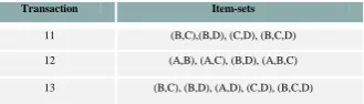
According to the first sub-problem we have to find the candidate item-set from the given database before generating the large/frequent item-set. So, from database, D the following candidates are taken along with their support (Table 2) using Eq no.(1).
Table 2: Candidate Item-set
Transaction Item-sets
11 (B,C),(B,D), (C,D), (B,C,D)
12 (A,B), (A,C), (B,D), (A,B,C)
13 (B,C), (B,D), (A,D), (C,D), (B,C,D)
Candidate Item-Set Support Candidate Item-Set Support
(A,B) 33% (B,D) 100%
(A,C) 33% (C,D) 67%
(A,D) 33% (A,B,C) 33%
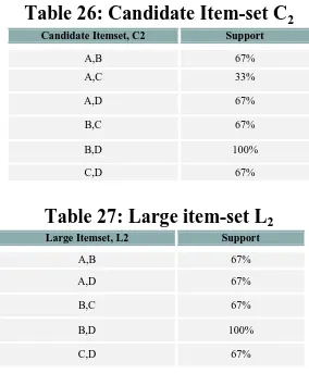
[image:2.595.344.517.695.756.2]Volume 78 – No.14, September 2013 As, we are provided with supmin=66%,
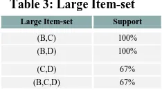
[image:3.595.113.230.97.162.2]Large item-set would be (Table 3).
Table 3: Large Item-set
Table 4: Possible Rules with Confidence
Step 2:
Next Step is to find the Association rules that can be generated from large item-set.
[image:3.595.118.214.450.515.2]For which we have to find the possible set of rules and their confidence (Table 4) using Eq no (2). And using given confmin=70%, Association Rules would be (Table 5).
Table 5: Association Rules
2.2
Algorithms for ARM
For ARM certain approaches/algorithms many have been proposed. Various among these algorithms are:
AIS Algorithm [13]:
The AIS algorithm is the first algorithm proposed for mining association rules. It is Adaptive Importance Sampling technique. The algorithm has two phases. The first phase constitutes the generation of the frequent item-sets. The algorithm uses candidate generation to detect the frequent item-sets. This is followed by the generation of the association rules in the second phase. The main drawback of the AIS algorithm is that it generates too many candidate item sets that need to be reduced, consuming more space and effort. This also requires too many passes over the whole database. These algorithms will be discussed in detail in section 3.
SETM Algorithm [6]:
SETM uses SQL to find large item-sets. The algorithm remembers TIDs i.e. transaction IDs of the transactions with the candidate item-sets. It uses this information instead of subset operation. This approach has a disadvantage that if Ck
needs to be sorted. And moreover if Ck is too large to fit in
buffer allocated memory space, the disk is used in FIFO approach. Then this requires two external sorts. These algorithms will be discussed in detail in section 4.
Apriori Algorithm [6,13]:
Apriori involves frequent item-sets, which is a set of items appearing together in the given number of database records meeting the user-specified threshold. Apriori uses a bottom-up search method that creates every single frequent item-set. This means that to produce a frequent item-set of length; it must produce all of its subsets as need to be frequent. This exponential complexity fundamentally restricts Apriori-like algorithms to discovering only short patterns. These algorithms will be discussed in detail in section 5.
FP-tree Algorithm [9,13]:
FP-tree-based algorithm is to partition the original database to the smaller sub-databases by using some partition cells, and then to mine item-sets in these sub-databases. Until no new item-sets are found, we have to recursively do the partitioning with the growth of partition cells. The FP-tree construction takes exactly two scans of the transaction database. The first scan collects the set of frequent items, and the second scan constructs the FP-tree.
Many other approaches have been introduced in between with minute changes. But main among them and which are basis for new upcoming algorithms are Apriori and FP-tree Algorithm. These algorithms will be discussed in detail in section 6.
3.
AIS ALGORITHM
In this approach candidate item-sets are generated and counted during the database scan [1]. It is done as follows:
After scanning transaction it is determined that which of the previously founded large item-sets are present in transaction.
New candidate item-set is generated by extending large item-sets in lexicographic order and their count entry is increased if it is created in previous transaction. Candidate item-sets are place in dynamic and multi-level hash table to make subset operation fast. When in case buffer overflow occur during candidate generation, the corresponding large item-set and its possible candidates is discarded from memory. The discarded large item-set discarded in pass are extended in next pass.
3.1 AIS Candidate and Large Item-set
The AIS function takes an argument L1, the set of all large
(1)-item-set and returns a superset of the set of all large k-item-sets. The function works as follows. First, in the extension step, we extend the frontier set. And in the pruning step, we don’t take those item-sets c, where c ϵ Ck such that
any (k-1)-subset of c is not in large item-setof the previous pass.
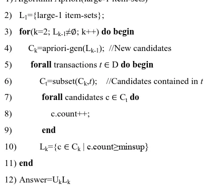
This whole process is defined using the algorithm 1 as follows:
1) Algorithm AIS (large-1 item-sets) 2) L1={large-1 item-sets};
3) for(k=2; Lk-1≠ ; k++) do begin
4) Ck= ;
5) forall transactions t D do begin
6) Lt=subset(Lk-1,t); //Large item-set contained in t
7) forall large item-sets lt Ltdo
8) Ct=1-extensions of lt contained in t
//Candidates in t Large Item-set Support
(B,C) 100% (B,D) 100% (C,D) 67% (B,C,D) 67%
Large Item-set Rules Confidence
(B,C)
B=>C sup(B∪C)/sup(B)=100/100=100%
C=>B sup(C∪B)/sup(C)= 100/100=100%
(B,D)
B=>D sup(B∪D)/sup(B)= 100/100=100%
D=>B sup(D∪B)/sup(D)= 100/100=100%
(C,D)
C=>D sup(C∪D)/sup(C)= 67/100 =67%
D=>C sup(D∪C)/sup(D)= 67/100 =67%
(B,C,D)
(B,C) =>D sup((B,C)∪D)/sup(B,C)= 67/100 =67%
(B,D) =>C sup((B,D)∪C)/sup(B,D)= 67/100 =67%
(C,D) =>B sup((C,D)∪B)/sup(C,D)= 67/67 =100%
Association Rules Confidence
Volume 78 – No.14, September 2013 9) forall candidates c Ctdo
10) if(c Ck) then
11) add 1 to count of c in corresponding entry in Ck;
12) else
13) add c to Ck with count of 1;
14) end
15) end
16) end
17) Lk={c Ck | c.count ≥ minsup}
18) end
19)Answer=UkLk
Algorithm 1: AIS Algorithm [1]
3.2 AIS Example
[image:4.595.73.267.63.202.2]AIS algorithm generates the candidate item-sets considering the transactions in the database. For Example; we are provided with a database D (Table 6) with some set of transactions, supmin=66% (i.e count=2) and confmin=70%
Table 6: Transaction Database, D
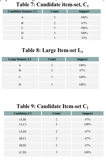
From Table 6 we find Candidate item-set (Table 7) and its support by the using Eq.no.1.
Next is to find the Large item-set, L1 using supmin=66%. i.e
Creating Table 8 from Table 7 using support threshold.
Step 1:
Candidate item-set C2 is generated by extending item-set L1
with only those items that are large and occur later in lexicographic ordering of items (Table 9 from Table 8).
[image:4.595.355.518.102.189.2]Table 7: Candidate item-set, C1
[image:4.595.77.236.271.318.2]Table 8: Large Item-set L1
Table 9: Candidate Item-set C2
Step 2:
Large item-set, Lk is generated from candidate item-set, Ck
using supmin. Large item-set L2 is created from Candidate C2
using support threshold.
The above two steps are repeated until Large Item-set came to be empty. i.e. From L2, candidate item-set C3 is generated
by extending it with only those items that are large and occur
later in lexicographic ordering of items (Table 11 to Table 10). The large item-set, L3 is same as candidate item-set, C3
as its support is more than support threshold.
Table 10: Large Item-set L2
Table 11: Candidate Item-set C3 and large item-set L3
At last candidate item-set, C4 cannot be generated further
from (A, C, D) and (B, C, D), as there is no other element in next lexicographic order to extend the large item-set L4.
4.
SETM ALGORITHM
SETM algorithm [1] uses same notation as used by other algorithms. But it uses SQL to compute large item-sets. It generates candidates as in AIS algorithm. To make use of standard SQL join process for candidate generation, it separates candidates from counting. Each member of these item-sets is of the form <TID, itemset>. It remembers TIDs of transactions with candidate item-sets. To avoid subset operation, the algorithm uses these TIDs to find large item-sets in transaction read. Ĉk is set of candidates in which TIDs
of generating transactions is associated. Here Ḹk C Ĉk and is
obtained by deleting the candidates not having minimum support. The disadvantage of SETM is that Ĉk needs to be in
sorted order. After counting and pruning the small candidate item-sets, resulting Ḹk needs to be sorted.
4.1 SETM Candidate and Large Item-set
The SETM function takes an argument L1, the set of all large
(1)-item-set and returns a superset of the set of all large k-item-sets. The function works as follows. First, the Ḹk and Ĉk
item-sets are created of the form <TID, itemset>. And the pruning step remains the same as of AIS i.e. we don’t take those item-sets c, where c ϵ Ck such that any (k-1)-subset of c
is not in large item-setof the previous pass.
This whole process is defined using the algorithm 2 as follows:
1) Algorithm SETM (large-1 item-sets) 2) L1={large-1 item-sets};
3) Ḹ1={large-1 item-sets together with sorted TIDs}
4) for(k=2; Lk-1≠ ; k++) do begin
5) Ĉk= ;
6) forall transactions t D do begin
7) Lt={l Ḹk-1 | l.TID = t.TID}; //Large (k-1)
item-set contained in t 8) forall large item-sets lt Ltdo
9) Ct=1-extensions of lt contained in t
//Candidates in t 10) Ĉk+={<t.TID, c> | l Ĉk };
11) end
12) end
13) Sort Ĉk on item-sets;
14) Delete item-sets c Ĉk for which c.count<supmin
Transaction Item-sets 11 (A,C), (A,D), (C,D), (A,C,D) 12 (A,B), (A,C), (B,D), (B,C,D)
13 (A,B), (A,D), (A,E), (B,C), (B,D), (C,D), (A,C,D), (B,C,D)
Candidate Itemset, C1 Count Support
A 3 100%
B 2 67%
C 3 100%
D 3 100%
E 1 33%
Large Itemset, L1 Count Support
A 3 100%
B 2 67%
C 3 100%
D 3 100%
Candidate,C2 Count Support
(A,B) 2 67%
(A,C) 3 100%
(A,D) 2 67%
(B,C) 2 67%
(B,D) 2 67%
(C,D) 3 100%
Large Itemset, L2 Count Support
(A,B) 2 67%
(A,C) 3 100%
(A,D) 2 67%
(B,C) 2 67%
(B,D) 2 67%
(C,D) 3 100%
Candidate Itemset, C3 and Large Itemset,
L3 Count Support
(A,C,D) 2 67%
[image:4.595.78.254.416.685.2] [image:4.595.337.543.593.755.2]Volume 78 – No.14, September 2013
giving Ḹk
15)Lk={l.itemset, count of t in Ḹk > l | l Ḹk };
16) end
17)Answer=UkLk
Algorithm 2: SETM Algorithm [1]
4.2 SETM Example
SETM algorithm generates the candidate item-sets considering the transactions in the database. For Example; we are provided with a database D (Table 12) with some set of transactions, supmin=66% (i.e count=2) and confmin=70%
Table 12: Transaction Database, D
Table 13: Item-set Ĉ1
From Table 12 we find create Ĉ1 using D (Table 13 using
Table 12).
Table 14: Large Item-set L1
Next is to find the Large item-set, L1 using supmin=66%. i.e
Creating Table 14 from Table 13 using support threshold.
Table 15: Item-set Ḹ1
Item-set Ḹ1 is created with the help from L1 and Ĉ1 (i.e Table
15 from Table 13, 14)
Step 1:
Candidate item-set C2 is generated by extending item-set L1
with only those items that are large and occur later in lexicographic ordering of items (Table 16 from Table 14). In this step we also create Ĉ2 using C2 and Ḹ1 (Table 17 using
Table 16, 14).
Step 2:
Large item-set, Lk is generated from candidate item-set, Ck
using supmin. Large item-set L2 is created from C2 using
support threshold (Table 17 from Table 16).
In this step we also create Ḹ2 using L1 and D (Table 19 using
Table 17, 18).
The above two steps are repeated until Large Item-set came to be empty.
Table 16: Candidate Item-set C2
Table 17: Item-set Ĉ2
Table 18: Large Item-set L2
Table 19: Item-set Ḹ2
Using the same procedure as explained above in Step 1 and 2, we create C3,Ĉ3, L3 andḸ3.
Table 20: (a) Candidate Item-set C3 and (b) Item-set Ĉ3
At last candidate item-set, C4 cannot be generated further
from (A, C, D) and (B, C, D), as there is no other element in next lexicographic order to extend the large item-set L4. Thus
Ĉ4 and Ḹ4 cannot be generated also.
Table 21: (a) Large Item-set L3 and (b) Item-set Ḹ3
5.
APRIORI ALGORITHM
The Apriori algorithm [6] generate the candidate item-sets in a pass by using only the item-sets found large in the preceding pass without considering the transactions of the database. The basic concept it uses is that any subset of a large set must be large. Therefore, the candidate item-sets having k items can be generated from previous pass by joining large item-sets having k-1 items (candidate generation), and delete those that contain any subset that is not large (Pruning concept). The procedure resulted in generation of a much smaller number of candidate item-sets. Algorithm 3 is the Apriori algorithm. The first pass of the algorithm simply finds the item occurrences to determine the large 1-item-sets. A pass, say pass k, has two phases. First, the large item-sets, say Lk-1 founded in the (k-1)
th
pass are used to generate the candidate item-set Ck, using the
apriori-gen function discussed in Section 5.1. Then, the database is scanned and support of candidates in Ck is calculated. For
fast calculations, we need to efficiently determine the candidates in Ck that are contained in a given transaction t.
`TID Set of Item-set
11 { {A,C},{A,D},{C,D} }
12 { {A,B},{A,C},{A,D},{B,C},{B,D},{C,D}} 13 { {A,B},{A,C},{A,D},{B,C},{B,D},{C,D}}
TID Set of Item-set
11 { {A},{C},{D} }
12 { {A},{B},{C},{D} }
13 { {A},{B},{C},{D},{E} }
Itemset, L1 Count Support
A 3 100%
B 2 67%
C 3 100%
D 3 100%
TID Set of Item-set
11 { {A},{C},{D} }
12 { {A},{B},{C},{D} }
13 { {A},{B},{C},{D} }
Candidate,C2 (A,B) (A,C) (A,D) (B,C) (B,D) (C,D)
Transaction Item-sets 11 (A,C), (A,D), (C,D), (A,C,D) 12 (A,B), (A,C), (B,D), (B,C,D)
13 (A,B), (A,D), (A,E), (B,C), (B,D), (C,D), (A,C,D), (B,C,D)
Large Itemset, L2 Count Support
(A,B) 2 67%
(A,C) 3 100%
(A,D) 2 67%
(B,C) 2 67%
(B,D) 2 67%
(C,D) 3 100%
TID Set of Item-set
11 { {A,C},{A,D},{C,D} } 12 { {A,B},{A,C},{A,D},{B,C},{B,D},{C,D}} 13 { {A,B},{A,C},{A,D},{B,C},{B,D},{C,D}}
Candidate Itemset, C3 (A,B,C)
(A,B,D)
(A,C,D)
(B,C,D)
TID Set of Item-set
11 { {A,C,D} }
12 { {A,B,C},{A,B,D},{A,C,D},{B,C,D}}
13 { {A,B,C},{A,B,D},{A,C,D},{B,C,D}}
Large Itemset, L3 Count Support
(A,C,D) 2 67%
(B,C,D) 2 67%
TID Set of Item-set
11 { {A,C,D} }
12 { {A,C,D},{B,C,D}}
Volume 78 – No.14, September 2013 Section 5.2 describes the subset function used for this
purpose.
1)Algorithm Apriori(large-1 item-sets) 2) L1={large-1 item-sets};
3) for(k=2; Lk-1≠ ; k++) do begin
4) Ck=apriori-gen(Lk-1); //New candidates
5) forall transactions t D do begin
6) Ct=subset(Ck,t); //Candidates contained in t
7) forall candidates c Ctdo
8) c.count++; 9) end
10) Lk={c Ck | c.count≥minsup}
11) end
12)Answer=UkLk
Algorithm 3: Apriori Algorithm [6]
5.1 Apriori Candidate Generations [6]
The apriori-gen function takes an argument Lk-1, the set of all
large (k-1)-item-set and returns a superset of the set of all large k-item-sets. The function works as follows. First, in the join step, we join one Lk-1 with another matching Lk-1. And in
the next prune step, we delete those item-sets c, where c ϵ Ck
such that any (k-1)-subset of c is not in Lk-1 of the previous
pass.
1) Algorithm Apriori-gen(Lk)
2) insert into Ck
3) select p.item1.p.item2,...p.itemk-1,q.itemk-1
from Lk-1 p,Lk-1 q
where p.item1=q.item1...p.itemk-2= q.itemk-2,
p.itemk-1<q.itemk-1;
4) forall item-sets c Ckdo
5) forall (k-1)-subsets s of c do
6) if(s Lk-1) then
7) delete c from Ck;
Algorithm 4: Apriori-Gen function [6]
5.2 Subset Function
Candidate item-sets Ck are stored in a hash-tree for use. A
node of this hash-tree either contains a list of item-sets (as leaf node) or a hash table (as interior node). In the interior node, each value in the hash table points to another node. If root is defined to be at depth 1, then the interior node at depth d points to nodes at depth d+1. Item-sets are stored in the leaf nodes. When we add a created item-set c from Apriori-gen function, we start from the root and go down the tree until we the leaf is reached. At the interior node of depth d, we decide which branch to follow by using a hash function to dth item of the item-set. When the number of item-sets in a leaf node exceeds the specified mentioned threshold, the leaf node is converted to make an interior node.
From the root node, the subset function finds all candidates contained in a transaction, t as described below:
If we are at leaf, we find which of the item-sets in this leaf are contained in t and add the references to them. If we are at interior node and we have reached it by hashing the item j, we apply hash function on each item coming after j in t and this procedure is applied to the node recursively.
5.3 Apriori Example
As Apriori algorithm generate the candidate itemsets without considering the transactions in the database, so firstly create database appropriate for Apriori i.e. from Table 22 to Table 23. For Example; we are provided with a database D (Table 23) with some set of transactions, supmin=66% and
confmin=70%
[image:6.595.71.275.97.285.2]Table 22: Database D
Table 23: Transformed Database
Before creating large item-sets (L1, L2, L3, L4 & so on) and
candidate item-sets (C2, C3, C4 & so on) candidate, firstly
Candidate item-set, C1 is generated from database (i.e. Table
24 from Table 23) and then, Large item-set, L1 is created
[image:6.595.352.505.396.515.2]from C1 using supmin=67% (i.e. Table 25 from Table 24)
Table 24: Candidate Item-set C1
Table 25: Large Item-set L1
Step 1:
Candidate set is generated as follows:
• The candidate itemsets, Ck can be generated by joining
large itemsets Lk-1 items, and
• Deleting those that contain any subset that is not large.
In Example C2 is generated from L1 items by join procedure
(i.e. Table 26 from Table 25) and those item-sets are deleted that have some (k-1) subset of c is not in Lk-1 where c Ck.
Step 2:
Large item-set, Lk is generated from candidate item-set, Ck
using supmin. Large item-set L2 is created from Candidate C2
using support threshold (Table 27 from Table 26).
The above two steps are repeated until Large Item-set came to be empty.
Here from the candidate item-sets, C2 elements with sup ≥
supmin, Large item-set, L2 is created (Table 27 from Table
26). As all candidate item-sets, C3 has sup ≥ supmin, so all
became Large item-set, L3 (Table 28 from Table 27).
Transaction Item-sets 11 (A,C),(B,D), (C,D), (B,C,D)
12 (A,B), (B,D), (A,B,D)
13 (B,C), (B,D), (C,D), (D,E), (B,C,D)
Transaction Items
11 A,B,C,D
12 A,B,D
13 B,C,D,E
Candidate Itemset, C1 Support
A 67%
B 100%
C 67%
D 100%
Large Itemset, L1 Support
A 67%
B 100%
C 67%
Volume 78 – No.14, September 2013
Table 26: Candidate Item-set C2
Table 27: Large item-set L2
[image:7.595.92.234.63.235.2]Table 28: Candidate Item-set C3 & Large item-set L3
Table 29: Candidate Item-set C4 & Large item-set L4
Same technique is used to create C4 and L4 (Table 29). As
all candidate item-sets, C4 has sup ≥ supmin, so all became
Large item-set, L4.
6.
FP-TREE APPROACH
This approach develops the three techniques in order to solve the problem of Apriori-like algorithm that may suffer in terms of cost to handle a huge candidate sets and repeatedly scanning the database for large set.
Compact data structure, called frequent-pattern tree, or FP-tree, is constructed, that stores information about frequent patterns. Only frequent length-1 items are making nodes in tree, and these nodes are arranged in a way that the more frequently used nodes must have better chances of node sharing than the less frequent items.
An FP-tree-based mining method is developed. Starting from a frequent length-1 pattern (as initial suffix pattern), examine only conditional-pattern or sub-database. The pattern growth is achieved using concatenation of the suffix pattern with new ones generated from a conditional FP-tree.
The search techniques employed in mining is a partitioning-based, divide-and conquers method.
6.1 Frequent Pattern Tree: Construction
A frequent-pattern tree (or FP-tree) is a tree structure which has following properties:
1. It contains root labeled as “null”, children as set of item-prefix sub-trees, and a frequent-item-header table.
2. Every node of item-prefix sub-tree has three fields: Item-name, its count, and node-link, where a. Item-name defines which item this node
represents,
b. Count defines the number of transactions represented by the path reaching this node, and c. Node-link links one node to the next node in the
FP-tree.
d. Every entry in the frequent-item-header table consists of two fields:
e. Item-name and
f. Head of node-link is pointer pointing to the first node in the FP-tree which carries the item-name).
Process or algorithm to construct a frequent-pattern tree has two steps, explained as follows:
Step 1:
A scan over database, D derives a list of frequent items of the form => (A:4), (C:4) and so on, in which items are ordered in frequency descending order, where the number after “:” indicates the support/count. This ordering is of importance here as path will follow this sequence in tree.
Step 2:
The “null” labeled root is created for a tree. The FP-tree is constructed by scanning the transaction database DB for the second time.
[image:7.595.351.520.283.333.2]Example: Assume an Example of Table 29. We can create FP-tree as defined in above steps.
Table 30: Transaction Table (Database, D)
Step 1:
Scan of the transactions one by one and construct list of item-sets as follows:
(A:4), (B:2), (C:4), (D:3), (E:3), (F:2), (G:1), (H:1) Here, (A:2) means A’s support= 2 and so on. And ordered frequent item-set would be if supmin=2 (i.e.
67%), then (A:4), (C:4), (D:3), (E:3), (B:2), (F:2)
Table 31: Frequent Items
Step 2:
Database is scanned second time to create FP-tree. Scan the first transaction to the construct of the first branch of the tree:
(A:1), (C:1), (D:1), (E:1), (B:1), (F:1)
Then move to second transaction. Since the transaction has common prefix (B, D, A) as with the previous one, they share the path and count of each node is incremented by 1 for these nodes as (B:2), (D:2), (A:2).
[image:7.595.327.506.430.512.2]The process is repeated to complete the FP-tree.
Figure 2: Frequent Pattern Tree
Candidate Itemset, C2 Support
A,B 67%
A,C 33%
A,D 67%
B,C 67%
B,D 100%
C,D 67%
Large Itemset, L2 Support
A,B 67%
A,D 67%
B,C 67%
B,D 100%
C,D 67%
Candidate itemset, C3 and Large Set L3 Support
A,B,D 67%
B,C,D 100%
Candidate itemset, C4 Support
A,B,C,D 67%
Transaction Items
11 A,B,C,D,E,F
12 A,C,D,E,F,H
13 A,B,C,E,G
14 A,C,D
Transaction Items Ordered Frequent Items
11 A,B,C,D,E,F A,C,D,E,B,F
12 A,C,D,E,F,H A,C,D,E,F
13 A,B,C,E,G A,C,E,B
14 A,C,D A,C,D
root
A: 4
C: 4
D: 3
E: 2
B: 1
F: 1
E: 1
F: 1
item
HEADER TABLE
A C D E B F
B: 1
[image:7.595.338.533.614.712.2]Volume 78 – No.14, September 2013
6.2 Mining Frequent Pattern with FP-Tree
In order to mine the required frequent patterns from FP-tree efficiently, a technique was proposed called FP–growth. In this technique the mining is done by finding the Conditional Patter Base and Conditional FP-tree of the frequent items say, nodes.
Conditional Pattern Base for a frequent item is the list of items in sequence coming between the frequent item and the root.
Conditional FP-tree for a frequent item is the list of items common in all conditional pattern base of the frequent item.
The whole process for mining constitutes two steps:
Step 1:
Create the conditional pattern base for X. Then create FP-tree for the frequent item.
Step 2:
From the conditional FP-tree of the frequent item X construct frequent patterns containing X by pairing it with the other items coming in its conditional FP-tree.
The above two steps are repeated for all of the frequent items.
Example: Assume the same Example taken above in Table 29. We have constructed the FP-tree (Figure 2) for the given database. Now, we have to mine the frequent patterns that contain frequent item-set by the use of the process as defined above.
Step 1:
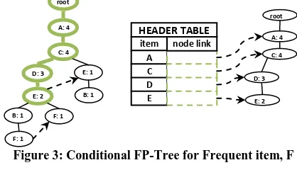
For node F, the immediate frequent pattern is (F:2), and it has two paths, {A:4, C:4, D:2, E:2, B:1, F:1} and {A:4, C:4, D:2, E:2, F:1}. So, F’s conditional pattern-base is {(ACDEB:1), (ACDE:1)}. We derive F’s conditional FP-tree, {(A:4, C:4, D:2, E:2)}|F as in Figure 3.
[image:8.595.57.266.452.572.2]Similarly, the conditional pattern base and conditional FP-tree is created for all other frequent items (as in Table 31).
[image:8.595.55.274.604.674.2]Figure 3: Conditional FP-Tree for Frequent item, F
Table 32: Conditional Pattern Base & Conditional FP-tree for all frequent items
Step 2:
This conditional FP-tree is then mined from ({A:4, C:4, D:3,E:2} | F). Figure 3 represents “({A:4, C:4, D:3, E:2} | F)” involves mining four items (A), (C), (D), (E) in the sequence. From this conditional FP-tree of the frequent item F, we construct frequent patterns containing F by pairing it with the other items coming in its conditional FP-tree.
We first derives a frequent pattern (EF:2), a conditional pattern-base {ACD:2}, and conditional FP tree for it would be ({A:2, C:2, D:2} | EF);
Secondly derives a frequent pattern (DF:2), a conditional pattern-base {( AC :2)}, and conditional FP tree for it would be ({A:2, C:2} | DF);
Thirdly derives a frequent pattern (CF:2), a conditional pattern-base {( A:2)}, and conditional FP tree for it would be ({A:2} | CF);
Then recursively derives other patterns (AF:2), (DEF:2), (CEF:2), (AEF:2), (CDF:2), (ADF:2), (ACF:2), (ACDF:2), (ACEF:2), (ADEF:2), (CDEF:2) and (ACDEF:2). Therefore, the set of frequent patterns involving F is: {(F:2), (EF:2), DF:2), (CF:2), (AF:2), (DEF:2), (CEF:2), (AEF:2), (CDF:2), (ADF:2), (ACF:2), (ACDF:2), (ACEF:2), (ADEF:2), (CDEF:2) and (ACDEF:2)}.
Table 33: Possible Frequent Patterns
Similarly, the possible frequent patterns are created for all other frequent items (as in Table 32).
7. CONCLUSION
The paper discussed the various main ARM approaches in detail. The various approaches discussed in this paper have many pros and cons. The AIS algorithm generates too many candidate item sets that consume more space/effort and also requires too many passes over the whole database. The SETM approach needs candidate item-set to be sorted and if it is too large to fit in buffer allocated memory space, the disk is used in FIFO approach. APRIORI involves frequent item-sets for candidate generation using a bottom-up search, which requires producing all of its frequent subsets. This results in exponential complexity not suitable for discovering bigger patterns. FP approach needs exactly two scans of the transaction database and avoids costly candidate generation. But this approach needs to whole procedure to be done again (i.e. generation of FP-tree, conditional pattern base, conditional pattern tree, etc).
Many other approaches have also been introduced for ARM with minute changes to the previous ones. But main among them which acts as basis for new upcoming algorithms are APRIORI and FP-tree Algorithm.
8. REFERENCES
[1] R. Agrawal, T. Imielinski, and A. N. Swami, 1993. Mining association rules between sets of items in large databases. ACM SIGMOD International Conference on Management of Data, Washington, D.C., pp 207-216. [2] U. Fayyad, G. Piatetsky-Shapiro and P. Smyth, 1996.
From data mining to knowledge discovery: an overview. Advances in Knowledge Discovery and Data Mining, MIT Press, Cambridge, MA.
Frequent Item Conditional Pattern Base Conditional FP-tree
A Ø Ø
C {(A:4)} {(A:4)} | C
D {(AC:3)} {(A:3,C:3)} | D
E {(ACD:2),(AC:1)} {(A:3, C:3)} | E
B {(ACDE:1),(ACE:1)} {(A:2, C:2)} | B
F { (ACDEB:1), (ACDE:1) } { A:2, C:2, D:2, E:2 } | F
Frequent Item Possible Frequent Pattern
A {(A:4)} C {(C:4), (AC:4)} D {(D:3), (CD:3), (AD:3), (ACD:3)} E {(E:3), (AE:3), (CE:3), (DE:2), (ACE:3), (ADE:2),(CDE:2),
(ACDE:1)}
B {(B:2), (AB:2), (CB:2), (DB:1), (EB:2), (ACB:2), (ADB:1), (AEB:2), (CDB:1), (CEB:2), (ACDB:1), (ACEB:2), (ADEB:1), (CDEB:1),
(ACDEB:1)}
F {(F:2), (EF:2), DF:2), (CF:2), (AF:2), (DEF:2), (CEF:2), (AEF:2), (CDF:2), (ADF:2), (ACF:2), (ACDF:2), (ACEF:2), (ADEF:2),
(CDEF:2) and (ACDEF:2)}
root
A: 4
C: 4
D: 3
E: 2
item
HEADER TABLE
A C D E
node link
root
A: 4
C: 4
D: 3
E: 2
B: 1
F: 1
E: 1
Volume 78 – No.14, September 2013 [3] U. Fayyad, S. G. Djorgovski and N. Weir, 1996.
Automating the analysis and cataloging of sky surveys. Advances in Knowledge Discovery and Data Mining, MIT Press, Cambridge, MA, pp. 471-94.
[4] 1997. Technology Forecast, Price Waterhouse World Technology Center, Menlo Park, CA.
[5] M. S. Chen, J. Han, and P. Yu, 1996. Data mining: an overview from a database perspective. IEEE Transactions on Knowledge and Data Engineering, vol. 8, no. 6, pp. 866-883.
[6] Rakesh Agarwal, Ramakrishna Srikant, 1994. Fast Algorithm for mining association rules. VLDB Conference Santiago, Chile, pp 487-499.
[7] S. A. Abaya, 2012. Association Rule Mining based on Apriori Algorithm in Minimizing Candidate generation. International Journal of Scientific & Engineering Research, vol-3, issue 7.
[8] Sotiris Kotsiantis, Dimitris Kanellopoulos, 2006. Association Rules Mining: A Recent Overview. GESTS International Transactions on Computer Science and Engineering, vol.32 (1), pp. 71-82.
[9] JaiWei Han, Jian Pei, Yiwen Yin & Runying Mao, 2004. Mining frequent patterns without candidate generation: A Frequent pattern tree approach. Data mining and knowledge discovery, Netherlands, pp 53-87.
[10]Huan Wu, Zhigang Lu, Lin Pan, Rong Seng XU and Wenbao jiang, 2009. An improved Apriori based
algorithm for association rule mining. IEEE Sixth international conference on fuzzy systems and knowledge discovery, pp 51-55.
[11]Farah Hanna AL-Zawaidah, Yosef Hasan Jbara and Marwan AL-Abed Abu-Zanana, 2011. An improved Algorithm for mining Association Rule in large database. World of Computer and Information technology, vol. 1, no. 7, pp 311-316.
[12]Zhuang Chen, Shibang Cai, Quilin Song, Chonglai Zhu, 2011. An Improved Apriori Algorithm based on pruning Optimization and transaction reduction. IEEE transactions on evolutionary computation, pp 1908-1911.
[13]Suhani Nagpal, 2012. Improved Apriori Algorithm using logarithmic decoding and pruning. International Journal of Engineering Research and Applications, vol. 2, issue 3, pp. 2569-2572.
[14]M. Suman, T. Anuradha, K. Gowtham, A. Ramakrishna, 2012. A frequent pattern mining algorithm based on FP-tree structure and Apriori algorithm. International Journal of Engineering Research and Applications, vol. 2, issue 1, pp.114-116.
[15]Sang Jun Lee, Keng Siau, 2001. A review of data mining techniques. Industrial Management and Data Systems, University of Nebraska-Lincoln Press, USA, pp 41-46.
![Figure 1: KDD process [15]](https://thumb-us.123doks.com/thumbv2/123dok_us/8065735.777801/1.595.317.564.421.597/figure-kdd-process.webp)