Environmentally sustainable economic dispatch using grey wolves optimization

ENVIRONMENTALLY SUSTAINABLE ECONOMIC DISPATCH USING

GREY WOLVES OPTIMIZATION

Kalyan Sagar Kadali

, Rajaji Loganathan

, Moorthy Veerasamy

and Viswanatharao Jawalker

1

Department of Electrical and Electronics Engineering, AMET University, Chennai, India

2_{ARM College of Engineering and Technology, Chennai, India} 3

Swarnandhra College of Engineering and Technology, Narsapur, India

4

Vallurupalli Nageswara Rao, Vignana Jyothi Institute of Engineering and Technology, Hyderabad, India E-Mail: [email protected]

ABSTRACT

This paper delineates a computational framework to ascertain optimum thermal generation schedule using newfangled grey wolves’ optimization (GWO) technique corresponding to environmentally sustainable, economic operation. This scheduling problem is devised as a bi-objective optimization and linear interpolated price penalty model is developed based on simple analytical geometry equations which blends two non-commensurable objectives perfectly. In order to obtain high-quality solutions within lesser executing time, the algorithm parameters are nicely replaced with system parameters that carry out global and local search process in the feasible region collaboratively. Further, an appropriate constraint handling mechanism is suitably incorporated in the algorithm that intern produces a stable convergence characteristic. The effectiveness of the proposed approach is illustrated on six unit thermal systems with due consideration of transmission line loss and valve point loading effect. The desired GWO technique reports a new feasible solution for quadratic and non-convex thermal operating model which is compared with the solution that has evolved earlier and the comparison shows that the GWO technique has outstripped other algorithms effectively.

Keywords: nonlinear and non-convex operating model, bi-objective optimization, economic-environmental impacts, gray wolves optimization, interpolated price penalty factor.

1. INTRODUCTION

Progressive economic dispatch: The world’s largest economy and fastest growing energy market mainly rely on the electricity from fossil fuel based thermal power plants. The twenty third issues of the Indian energy statistics report reveal that India holds fourth largest place on the world’s energy market, its electricity generation from utilities and non-utilities altogether during 2014-15 were 71.01%, 13.04%, 1.82% and 14.11% from thermal, hydro, nuclear and non-utilities respectively. The thermal power plant shares more proportion on the total generation and the emission released during production causes inevitably dominance impact of environmental. With the increased concern over environmental protection, the power industries are forced to modify their operation strategies for the generation of electrical energy not only at minimum energy cost, but also at minimum pollution level to meet the requirements of the increasing demand [1-2]. Further, it has been recognized that the energy utilization improvement and environmental impact assessment are an essential step to achieve sustainable development of a country. With its rapid economic up growth, the rising energy consumption as well as environmental pollution has been impelling the researchers to derive a strategic balance between economic development, energy consumption and environmental sustainability [3].

Economic dispatch (ED) is a cognitive process that optimizes the power generation intent to minimize the total operating cost and to meet load demands over a schedule period while satisfying the various equality and inequality constraint. Due to the apprehension over environmental pollution and clean air amendment forces the utilities to serve electricity, cheapest possible price

with cleanliness environment. Hence, the ED now becomes an environmentally constrained economic dispatch problem (ECED).

1.1 State-of-the-art literature

The literature survey basically focused on economic load dispatch (ELD) and combined economic-emission dispatch (CEED) in thermal power systems. This review covers three methodologies based classification such as classical, meta-heuristic and hybrid optimization techniques.

Classical optimization techniques: Over the past decades, a number of conventional approaches were applied for solving the ED problem. In which, direct Newton–Raphson [4], branch-and-bound [5] and interior point methods [6] have been addressed solution for ELD problem. Likewise, Lagrangian relaxation [7] and back propagation neural network (BPNN) [8] methods were found solution to CEED. Despite, classical methods have found an accurate solution; it uses a single path search method based on the deterministic transition rule, while searching the optimal solution in the search space. Hence, these methods have taken the more computational time and have occupied more memory space.

differential evolution (MODE) [13] have optimized both fuel cost and emission simultaneously. In fact, the convergence rate of opposition-based harmony search (HS) [15], tribe-modified differential evolution (Tribe-MDE) [16] and self-organizing hierarchical particle swarm optimization technique with time-varying acceleration coefficients (SOHPSO TVAC) [17] are fine-tuned while optimizing CEED problem by modifying the operator.

Hybrid optimization methods: In the scenario of optimization process a strategic balance between global and local search are derived by combining either two heuristic algorithms or one heuristic algorithm with a classical method. The hybrid PSO with the sequential quadratic programming (PSO-SQP) [18] technique, modified sub-gradient and harmony search (MSG-HS) algorithm [19] and hybrid shuffled DE (SDE) algorithm [20] have obtained good quality solution for ELD problem. Moreover, the hybrid genetio algorithm [22] modified neo-fuzzy neuron (NFN) [23], GA with active power optimization based on Newton’s second order approach [24] and differential evolution and biogeography-based optimization (DE-BBO) algorithm [25] have determined compromised generation schedule in CEED case.

1.2 Research gap and motivation

However, the reported optimization techniques had found optimum solution; it is not an end global solution to ELD problem due to the common shortcomings of algorithm complexity, premature convergence due to imbalance between exploration and exploitation, and large computational time. To overcome this drawback, a new emerging optimization tool, i.e., grey wolves optimization (GWO) technique is preferred with suitable constraint handling strategy, which balances intensification and diversification through encircling, hunting and attacking processes. Then, superior convergence characteristics and performance of the GWO technique than other swarm intelligence techniques while solving economic load dispatch problem with only fuel cost as objective function [26] - [27] and the unit commitment problem [28] have been successfully analyzed.

1.3 Highlights of this work

As far as the state of the art, literature, there has been no attempt to demonstrate the emission constrained economic operation of thermal power system with valve point loading using GWO. Therefore, ascertaining the preeminent generation schedule for compromised fuel cost and emission release with less computational time is still a research work. This motivates the authors to contribute in this research field in the following aspects:

 The six unit thermal power system’s data are suitably incorporated into the coded GWO technique.

 A linear interpolation model is proposed to blend the fuel cost and emission releases.

 A benchmark emission constrained economic generation schedule is derived using GWO technique; it seems to be the first attempt.

1.4 Paper organization

The paper is organized into six sections, the next section describes the mathematical formulation of the emission constrained economic dispatch problem, whereas, section 3 deals GWO technique as an optimization tool is briefed. Section 4 deals application of GWO’s technique for finding an optimal generation schedule. The numerical simulation results are presented and have compared in section 5. Finally, the conclusion is presented in the last section.

2. EMISSION CONSTRAINED ECONOMIC DISPATCH MODEL

2.1 Objective functions

As stated earlier the ECED problem is formulated as a bi-objective framework, and is described mathematically as follows:

Minimize





1

( ) , ( ) N

gi gi

i

F P E P





(1) Where, Pgi is active power generation (MW) of ith

unit, F and E are total fuel cost (FC) of generation in the system (Rs./hr) and emission release (kg/hr) respectively and N is the number of thermal units.

Cost function:Revenue analysis of utility relies linear, quadratic and cubic cost functions. If a cost function is said to be an economically meaningful and legitimate that it should be satisfied the restriction imposed by the parameter and variable. In case of quadratic cost function there are three restrictions to be satisfied where as the cubic cost function need to satisfy additionally one inequality restriction. Moreover, one of the quandaries of cubic cost function should be hypothesized. Therefore, economists are chosen quadratic cost function either maximize profit maximum or minimize operating cost. Particularly, the total fuel cost of thermal plant is expressed sum of multiple quadratic cost function in terms of real power generation and is mathematically defined as follows:





1

( ) N

gi i gi i gi i

i

F P a P b P c







(2) where, ai bi and ci are the fuel cost coefficients of the ith generating. The significant effect of valve point loading on total FC can be pragmatically designated as the superposition of quadratic and sinusoidal function. The total generation cost with valve point loading is given by:













2

1

min

( )

sin

N

gi i gi i gi i

i

i i gi gi

F P a P b P c

d e P P



  

 



(3)

where, diand ei are the coefficients of the effect

Emission function: The emission generated by each generating unit may be approximated as a quadratic function of the power output of the generator. The total amount of emission released is given by:

 

gi i i gi i gi

E P   P  P (4)

where, i i and i are the emission coefficients of the ith unit.

2.2 Handing bi-objective

The bi-objective problem of emission constrained economic dispatch (ECED) can be converted into the single objective optimization problem by introducing a normalized price penalty factor. The price penalty factor is defined as the ratio between the average full load fuel cost and average emission of the corresponding generator as its maximum output.

a) Computation of modified price penalty factor Step 1: The computation ofhmax:









max max

max _{max max}

gi gi

gi gi

F P P

h

E P P

 (5)

Step 2: According to hmax the thermal units were ranked in ascending order.

Step 3: Then full-load capacity of each unit was added one at a time starting from the lowest hmaxuntil

max



Step 4: In this procedure hmaxrelated to last unit was considered as a price penalty factor to trade-off two conflict objectives.

b) Computation of normalized price penalty factor

While performing step 3 sum of the maximum capacity of thermal units often greater than demand, it may lead approximate value. In order to determine the no-inferior solution an accurate model is necessary which is not explored in the literature. This drawback can be rectified by incorporating a simple mathematical technique with the usual procedure. Let, P_g1 is the maximum capacity of a unit at that moment by adding the same causes sum total exceeds the load demand PD and its

corresponding price penalty factor is h1. The maximum

capacity Pgo is the predecessor and the associated price

penalty is ho. Then the normalized price penalty factor (ht)

can be determined using (6).





1

1

*

o

t o D go

g go

h h

h h P P

P P

 _   _ _ 



  (6)

Now, the objective function has detailed in (1) can be defined by introducing ht, then the objective

function of ECED problem is defined as,

Minimize





2.3 Constraints

a. Equality constraint

The algebraic sum of the total generated power of all generating units, power demanded by the load and the total transmission loss (PL) must be equal to zero.

1

0

N

gi D L

i

P P P



  



The Kron’s loss formula is given by:

,0 00

1 1 1

N N N

L gm mn gn m gm

m n m

P P B P B P B

  







where, Bmn, Bmo and Boo are the elements of loss coefficient matrix.

b. Inequality constraint

The power output of each generating unit must be greater than or equal to the minimum power permitted and also be less than or equal to maximum power permitted on that specified unit. Thus the inequality constraint is expressed as:

min max

1, 2,....

gi gi gi

P P P i N

(10)

where,

min ,

gi

P max

gi P

are the minimum and maximum power generation limit of the the ithunit.

3. OVERVIEW OF GWO TECHNIQUE

It is a population based metaheuristic algorithm and developed by Mirjalili et al., in 2014 which is inspired from the leadership hierarchy and the hunting mechanism of gray wolves in nature. Generally, the populations of grey wolves have average crowd size of 5-12 and the cluster organizes compactly through the hierarchy. The most dominant member is called alpha; the immediate successive ranked wolves are beta, delta and omega in which beta supports in decision making whereas delta lead its lowest rank.

individual grey wolf adjusts its position and moves to the best position, and the best feasible solution in the course of the iteration is saved.

The mathematical formulation of the GWO is carried through the following segments to determine the best feasible solution for any optimization problem.

 Encircling

 Hunting

 Attacking

The encircling behavior of the grey wolves is mathematically represented s follows.

 

 

p

D C X t X t uur ur uur uur

(11)





 

X t X t  A D

uur uur ur uur

(12)

where, 𝑡 indicates the current iteration, urA and Cur

are coefficient vectors, uurXp is the position vector of the prey, and uurX indicates the position vector of a grey wolf. The vectors urA and Cur are calculated as follows:

1

2 A a r a

ur r r r

(13)

2 2

Cur rur (14)

where, 1 r

r and 2

ur

r are random vectors between 0 and 1 and ar is set to decrease from 2 to 0 over the course of iterations.

In the course of iterations the position of alpha seems to be considered as first best candidate solution and another two are beta and delta wolves’ position, and then the other search agents (omega wolves) update their positions according to the position of three best search agents. It can be modeled mathematically as follows:





 

 

 

1

3

X t X t X t

X t   

uur uur uur

uur

(15)

Where,

 

1 ₁

X X A D

uur uur uur uur

; D C1XX uur ur uur uur

(16)

 

2 ₂

X XA  D

uur uur uur uur

; D C2XX uur ur uur uur

(17)

 

3 ₃

X XA  D

uur uur uur uur

; D C3XX uur ur uur uur

(18)

Over the course of iterations the value of ar has decreased linearly from 2 to 0, thus urA also decreased byra

. As urA is fluctuating randomly in between the range [-a, a]

the candidate solution is converged towards prey if 1 ur

A

that means forcing the wolves to attack the prey otherwise forces the wolves to search another best candidate solution (alpha) and this process repeats till the termination criterion is fulfilled.

4. APPLICATION OF GWO TECHNIQUE FOR ECED

Step 1: Initialization and structure of candidate solution: The active thermal power generation is a control variable that representing the position of the wolves to be evolved. This is randomly engendered within the operational limits based on (19).





, *

g i gi gi gi

P rand P P P (19)

Then, the initial population matrix is created as follows:

1 1 1 1

1 2

2 2 2 2

1 2 1 2 . . . . . . . . . . . . . .

g g gi gN

g g gi gN

SP SP SP SP

g g gi gN

P P P P

P P P P

X

P P P P

                 (20)

Then, the initial position of the candidate solution Xo is initialized as follows.

1 1

1 1 2 2

1 1

..

.. ...

o SP SP

g g g g

SP SP

gi gi gN gN

X P P P P

P P P P



_     

    _ (21)

Step 2: Estimation of augmented objective function: From the initial position of the population the objective function is calculated. In order to handle equality constraint violation an augmented objective function (AOF) is derived using (22), which is the aggregate of the objective function considered and absolute value in violation of power balance constraint with a high valued scalar multiplier. Further, this mechanism converts the primal constrained problem into an unconstrained problem and guides the search process towards the desirable solution





1

1000* N

gi D L

i

AOF objective P P P



 

    





(wolf’s) distance from the prey. Sort the population from minimum to maximum, an individual having the minimum fitness is imitated as the alpha; second and third minimum is beta and delta respectively.

Fitness = AOF (23)

Step 4: Modifying agent position for optimal solution: The position of the ith agent should be updated in accordance with (15). The position of each search agent represents a potential solution comprised of an active power generation of ELD problem. The new position of each agent may violate allowable ranges and it is limited to the respective range.

Step 5: Fitness re-estimation: With the new position of each control variable, the AOF is calculated as described in the steps 2 and followed step 3 is performed to identify a global best solution.

Step 6: Modification of thermal generation schedule: The N-1 thermal generations are retained at the optimum value and one thermal generation, i.e., dth is modified to satisfy the power balance equation based on solution repair strategy. It can be solved using standard algebraic method and the positive root is chosen as the generation of the slack thermal unit that satisfies the equality constraint (8), perfectly.

    

   

1 1 1

2

,

1 1

1 1

,0 00

1 1

2 1

0

N N N

dd g d d m m g d m mn n

m m n

N N

m m m D

m m

m d

B P B P P P B P

B P P B P

  

 

 

 



  

_  _ _

  

 

    

 



 





(24)

Step 7: Inequality constraints handling mechanism: The decision variables of thermal plant output power are kept in the valid range by handling appropriately. Generally, it can be checked whether the operating limits of the active power of all generating units are violated or not. If any power generation is less than the minimum level, it is made equal to the minimum value. Similarly, if it is greater than the maximum level, it is assigned its maximum value.

Step 8: Stopping criterion: If_iter max_{Cycle, go to} step 2. Otherwise, the GWO terminates.

5. SIMULATION RESULTS AND DISCUSSION

5.1 Description of test system

The environmentally constrained economic operation of thermal plants is mathematically formulated as an optimization problem. A standard test system consists of six units is considered to investigate the performance of the GWO. The coefficients of cost and

emission characteristics, generator operating limits are referred from [17]. The operation is performed for 500MW, 700MW and 900MW static load. Initially, ECED is carried for nonlinear quadratic operating model further; the complexity of the dispatch model is increased by considering non-convex operating model. In the both model network line losses are considered and the loss coefficients are taken from the reference [11]. The GWO algorithm is coded in MATLAB 7.9 platform and is executed on Intel core i5 processor 2.30 GHz and 4 GB RAM personal computer.

5.2 Economic operation

The applicability of the GWO method for finding the optimum operation of thermal power system has been explored by analyzing two operating models, one is nonlinear quadratic operating cost model (module-I) whereas, the second is a non-convex operating model (module-II). In both the model fuel cost is considered as objective function and the algorithm is executed 500 repetitive iterations with same control parameters. Simulated optimum generation schedule of modules-I and II corresponding to the minimum fuel cost per hour are presented in Table-1 and Table-2 respectively. These tables mainly consist of generation schedule in MW and computational time in second for 500MW, 700MW and 900MW.

Table-1. Economic generation schedule for quadratic cost model.

Unit (MW) Demand (MW)

500 700 900

P1(MW) 10.0000 10 80.62866

P2(MW) 17.1430 15.28374 122.7474 P3(MW) 118.198 147.7319 205.3744 P4(MW) 55.2233 129.4321 57.41022 P5(MW) 183.7044 227.8039 248.9675 P6(MW) 125.2857 188.7093 212.2364 Total Generation

(MW) 509.5542 718.961 927.3646 Losses (MW) 9.54982 18.95229 27.90137

CPU Time(s) 8.8 10.90 11.18

Iterations 500 500 500

Fuel Cost (Rs/h) 27592.91 37013.08 48956.81 Emission

release(Kg/h) 296.2263 506.5107 775.9482

Table-2. Economic generation schedule for non-convex cost model.

Unit (MW) Demand (MW)

500 700 900

P2(MW) 10.0000 91.7526 147.6529

P3(MW) 108.7219 72.3733 62.5472

P4(MW) 55.8396 66.0208 99.2741

P5(MW) 130.0000 289.7264 292.1672 P6(MW) 195.5236 154.6388 284.9222

Total Generation

(MW)

510.0851 718.1385 930.9836 Losses

(MW) 10.084 18.3917 30.9682

CPU

Time(s) 10.91 10.73 10.77

Iterations 500 500 500

Fuel

Cost(Rs/h) 27767.4390 38172.5163 49376.4905 Emission in

(Kg/h) 301.4472 541.7688 835.1272 Additionally, the emission release (kg/hr) associates with this generation schedule also presented for better understanding. It is perceived from both the tables that the generation of each unit is within its operating limits and the fuel cost is increased while considering valve point loading.

5.3 Minimum emission operation

The potentiality of the GWO in minimizing pollutant emission release that has supplemented with the thermal power generation is examined for the stated modules in section 5.2 with same MW load. The algorithm is converged at acceptable pollutant emission level (kg/hr). Consequent optimum generation schedule and computational time are tabulated for nonlinear quadratic model in Table 3 and non-convex operating model in Table-4. From the test results it is understood that the GWO has curtailed the emission release in greater extent and the stated objective, i.e., minimum pollutant emission is achieved without violating the power generation limits to meet stipulated load demand.

Table-3. Generation schedule of quadratic cost model for minimum emission.

Unit (MW) Demand (MW)

500 700 900

P1(MW) 10 20.71155 112.6034

P2(MW) 29.18051 107.8707 145.1237 P3(MW) 76.09383 135.4213 148.3091 P4(MW) 106.6669 124.8187 118.4906 P5(MW) 157.1404 166.8462 200.3894 P6(MW) 132.2234 160.1151 202.0595 Total Generation

(MW) 509.305 715.7836 926.9757

Losses (MW) 9.305 15.783 26.975

CPU Time(s) 11.58 11.49 12.36

Iterations 500 500 500

Emission release

(Kg/h) 272.4754 455.8172 688.0668 Fuel Cost(Rs/h) 28044.2100 38147.59 49957.45

Table-4. Generation schedule of non convex cost model for minimum emission.

Unit (MW) Demand (MW)

500 700 900

P1(MW) 34.79092 84.70206 119.2070 P2(MW) 80.67597 110.8959 145.4126 P3(MW) 74.91931 116.0293 125.9743 P4(MW) 62.69852 80.90215 117.6297 P5(MW) 130.2411 159.4576 196.1398 P6(MW) 125.0057 164.259 223.1910 Total Generation

(MW) 508.3315 716.246 927.5545 Losses (MW) 8.331 16.246 27.5544

CPU Time(s) 11.09 11.14 11.35

Iterations 500 500 500

Emission release

Kg/h) 274.0989 445.0791 691.5438 Fuel Cost (Rs/h) 28461.63 38942.16 50290.1141

5.4 Emission constrained economic dispatch

Simulation results that were discussed in sections 5.2 and 5.3 reveals the conflict nature of fuel cost and emission release, i.e., while minimizing fuel cost alone the corresponding emission release increases in unacceptable value whereas, the fuel cost would be more while minimizing emission release separately.

Table-5. Generation schedule of quadratic cost model for compromised optimum solution.

Unit (MW) Demand (MW)

500 700 900

P1(MW) 10 20.71155 102.3468

P2(MW) 29.30387 107.8707 139.6853 P3(MW) 95.78365 135.4213 91.4198 P4(MW) 64.88712 124.8187 123.6492 P5(MW) 159.5717 166.8462 251.5216

P6(MW) 149.872 160.1151 219.7210

Total Generation

(MW)

509.4183 715.7836 928.3437 Losses

(MW) 9.4175 16.22349 28.4896

CPU

Time(s) 11.06 12.12 11.55

Iterations 500 500 500

Fuel Cost

(Rs/h) 27596.5500 38147.5900 49527.7400 Emission

release (Kg/h)

277.4680 455.8172 716.5007

Table-6. Generation schedule of non-convex cost model for compromised optimum solution.

Unit (MW) Demand (MW)

500 700 900

P1(MW) 10 26.1386 107.5265

P2(MW) 46.32485 105.6768 145.9959

P3(MW) 54.46726 79.5960 106.8263

P4(MW) 94.67492 62.3800 105.2623

P5(MW) 160.1301 254.6463 273.2420 P6(MW) 143.7522 189.6015 189.4708

Total Generation

(MW)

509.3493 718.0391 928.3237 Losses

(MW) 9.3620 18.9926 28.1511

CPU

Time(s) 11.06 11.4 11.87

Iterations 500 500 500

Fuel

Cost(Rs/h) 27742.5600 38287.2145 50038.1070 Emission

release (Kg/h)

280.1733 516.8659 725.9556

5.5 Feasible solution

In order to reveal the superiority of the GWO technique in solving emission, economic, and emission constrained economic operation of nonlinear thermal model, the simulated results are compared with SOHPSO [17] in Table-7. From the comparison, it is noticed that the proposed technique has saved fuel cost 487.07 Rs. /hr, 1194.92 Rs./hr and 350.13 Rs./hr for 500MW, 700MW and 900MW respectively, emission release has reduced 3.15kg/hr, 25.23 kg/hr and 62.7kg/hr for 500MW, 700MW and 900MW respectively than SOHPSO [17]. During the compromised operation, fuel cost saving and emission release reduction are 487.07Rs./hr & 0.0kg./hr for 500MW, 671.33 Rs/hr & 50.6935 kg/hr for 700MW and 600.03Rs/hr& 43.09kg/hr than SOHPSO [17].

Table-7. Comparison of feasible solution of GWO with SOHPSO for quadratic cost model.

Demand

(MW) Objective

SOHPSO [17] Proposed method

Pure ELD Pure ED ECED Pure ELD Pure ED ECED

500 FC (Rs./hr) 28,079.97 28,379.90 28,379.90 27592.90 28044.21 27596.55

ER (kg/hr) 310.13 276.55 276.55 296.23 273.4 277.468

700 FC (Rs./hr) 38,208.00 39,444.32 38,818.92 37013.08 38481.19 38147.59

ER (kg/hr) 536.77 462.90 468.35 506.5107 443.12 455.8172

900 FC (Rs./hr) 49,306.94 50,971.84 50,127.87 48956.81 49957.45 49527.74

ER (kg/hr) 845.11 750.77 759.59 775.9482 688.07 716.50

Table-8. Comparison of feasible solution of GWO for quadratic and non-convex cost models.

Demand

(MW) Objective

GWO’s solution for quadratic cost model

GWO’s solution for non-convex cost model

Pure ELD Pure ED ECED Pure ELD Pure ED ECED

500 FC (Rs./hr) 27592.90 28044.21 27596.55 27767.43 28461.63 27742.56

700 FC (Rs./hr) 37013.08 38481.19 38145.29 38172.52 38942.16 38287.22

ER (kg/hr) 506.51 443.12 455.82 541.77 445.07 516.87

900 FC (Rs./hr) 48956.81 49957.45 49527.74 49376.4905 50290.11 50038.11

ER (kg/hr) 775.94 688.07 716.50 835.13 691.54 725.96

In case of non-convex operating model, most of the researches have followed different load schemes. For uniqueness, the performance of GWO in solving non-convex and nonlinear operating model for all operations with same load demand has been compared in Table 8. The inclusion of valve point loading of thermal plant leads to multiple minima’s in the search space. Thus, the fuel cost is raised 174.53 Rs/hr, 1159.44Rs/hr and 419.68Rs/hr for 500MW, 700MW and 900MW respectively, in the case of emission dispatch the pollutant emission has increased 0.69 kg/hr, 1.95kg/hr and 3.47kg/hr for 500MW, 700MW and 900MW respectively than without valve point loading. Similarly, in the case of compromised dispatch the fuel cost 146.01 Rs/hr, 141.93 Rs/hr and 510.37 Rs/hr, and emission release 2.7kg/hr, 61.05 kg/hr and 9.46 kg/hr have been increased than without valve point loading for 500MW, 700MW and 900MW respectively.

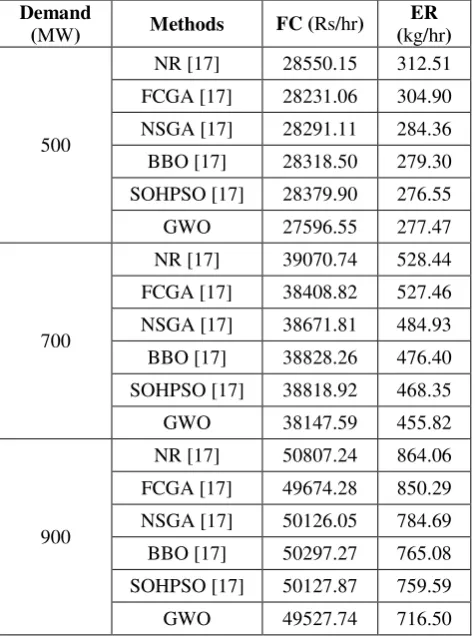
To show the diversity in comparison of emission constrained economic operation of nonlinear thermal unit, the compromised fuel cost and emission release have been compared with NR [17], FCGA [17], NSGA [17], BBO [17] and SOHPSO [17] inTable 9 for 500MW, 700MW and 900MW. The GWO has obtained better compromised fuel cost and emission reduction than other contestant algorithms, but there is no significant pollutant emission reduction as compared with SOHPSO [17] for 500MW. If SOHPSO is trying to minimize fuel cost further the corresponding emission release will be certainly greater than what the GWO technique has obtained.

5.6 Solution quality

The GWO algorithm is used for determining the optimum operation setting of thermal power system, the optimum values and feasible solution for different case studies have been presented in the previous sections. Generally, the solution quality can be explored by comparative analysis; therefore the feasible solutions for all operations over twenty trials are statically analyzed and the test results are presented in Table 10. It is noticed that the GWO technique is the best in minimizing fuel cost, emission release and compromised solution for 700MW load. Moreover, lower standard deviations of GWO shows the average and worst values are very close to its best value and also is ranked first in optimizing consider objective function.

Table-9. Comparison of compromised feasible solution of quadratic cost model.

Demand

(MW) Methods FC (Rs/hr)

ER (kg/hr)

500

NR [17] 28550.15 312.51 FCGA [17] 28231.06 304.90 NSGA [17] 28291.11 284.36 BBO [17] 28318.50 279.30 SOHPSO [17] 28379.90 276.55

GWO 27596.55 277.47

700

NR [17] 39070.74 528.44 FCGA [17] 38408.82 527.46 NSGA [17] 38671.81 484.93 BBO [17] 38828.26 476.40 SOHPSO [17] 38818.92 468.35

GWO 38147.59 455.82

900

NR [17] 50807.24 864.06 FCGA [17] 49674.28 850.29 NSGA [17] 50126.05 784.69 BBO [17] 50297.27 765.08 SOHPSO [17] 50127.87 759.59

GWO 49527.74 716.50

Figure-1. Convergence characteristics of GWO for economic generation schedule (Module-I).

Figure-2. Convergence characteristics of GWO for minimum emission (Module-I).

From Table-10 it is observed that the GWO technique has determined best fuel cost and minimum emission release, and also can be stated that both are conflicting nature. Thus, the trade-off between them is achieved using linear interpolated normalized price penalty factor approach. Figures 3 - 5 shows the optimal fronts that have obtained by the GWO technique for twenty independent trials for 500MW, 700MW, 900MW respectively, where the optimal fronts for both cases, i.e., nonlinear and non-convex cost model are compared. The trade-off curve confirms that GWO technique is nicely compromised fuel cost and emission release.

Table-10. Statistical comparison of feasible solution for the demand 700 MW.

Attribute Methods ELD ED ECED

FC (Rs/hr) ER (kg/hr) FC (Rs/hr) ER (kg/hr)

Best SOHPSO [17] 38208.00 462.90 38818.92 468.35

GWO 37013.08 443.12 38147.59 455.81

Average SOHPSO [17] 38208.56 463.24 38819.15 469.25

GWO 37013.50 443.98 38147.59 456.22

Worst SOHPSO [17] 38210.00 464.32 38820.84 470.00

GWO 37015.01 444.48 38149.45 457.22

Std. Dev. SOHPSO [17] 1.41 1.00 1.36 1.17

GWO 1.36 0.96 1.32 1.00

0 100 200 300 400 500

2 3 4 5 6 7 8 9 10x 10

4

Iterations

F

u

e

lc

o

st

(

R

s.

/h

r)

PD=500MW PD=700MW PD=900MW

0 100 200 300 400 500

200 400 600 800 1000 1200 1400 1600 1800 2000

Iterations

E

m

is

si

o

n

r

e

le

a

se

(

k

g

/h

r)

Figure-3. Comparison of optimal trade-off solution obtained by GWO for 500MW.

Figure-4. Comparison of optimal trade-off solution obtained by GWO for 700MW.

Figure-5. Comparison of optimal trade-off solution obtained by GWO for 900MW.

6. CONCLUSIONS

Economic and environmentally sustainable operation of thermal power system offers tough challenges to the researchers; hence the ELD problem is formulated as a bi - objective framework. Initially, fuel cost and emission release are optimized separately using a GWO technique whereas, the interpolated price penalty approach has been employed and optimized the objective functions simultaneously. The optimum generation schedule that has been obtained by GWO technique perfectly met the specified load demand. The simulated results have been compared with earlier research work. Therefore, it is concluded that the proposed algorithm can be robust and effective alternative for solving bi-objective economic load dispatch problem without and with valve point loading effect. Further, provides solution to serve electricity in affordable price with the cleanliness environment to the society. Finally, the numerical results would be useful for regulatory bodies, policy makers and power system planners.

ACKNOWLEDGEMENT

The authors would like to thank Shri Vishnu Engineering College for Women, Bhimavaram, Andhra Pradesh, India for providing infrastructural facilities to conduct the research work.

REFERENCES

[1] Ministry of statistics and programme implementation, Government of India, 138 Energy Statistics, New Delhi, India: Central Statistics Office. Available at: http://mospi.nic.in/mospi_new/upload/energy_stats_1 38_19mar8.pdf.

2.74 2.76 2.78 2.8 2.82 2.84

x 104 265

275 285 295 305

500MW

Fuel cost (Rs/hr)

E

m

is

si

o

n

r

e

le

a

se

(

k

g

/h

r)

Non convex cost model Quadratic cost model

3.7 3.8 3.9 4 4.1 4.2

x 104 460

500 540 580 620 660

700MW

Fuel cost (Rs/hr0

E

m

is

si

o

n

r

e

le

a

se

(

k

g

/h

r)

Non-convex cost model Quadratic cost model

4.8 5 5.2 5.4 5.6

x 104 650

700 750 800 850 900

900MW

Fuel cost (Rs/hr)

E

m

is

si

o

n

r

e

le

a

se

(

k

g

/h

r)

[2] Sudhir Y and Rajiv P. 2014. Status and environmental impact of emissions from thermal power plants in India. In: Environmental Forensics. 15: 219-22. [3] Bi G., Wen S., Zhou P., and Liang L., 2014. Does

environmental regulation affect energy efficiency in China's thermal power generation? Empirical evidence from a slacks-based DEA model. In: Energy Policy. 66: 537-546.

[4] Lin C.E., Chen S. T. and Huang C.L. 1992. A direct Newton-raphson economic dispatch. In: IEEE Transactions on Power Systems. 7(3): 1149-1154. [5] Chem-Lin C. and Shun-Chung W. 1993.

Branch-and-bound scheduling for thermal generating units. In: IEEE Transactions on Energy Conversion. 8(2): 184-189.

[6] Sergio G. 1994. Optimal reactive dispatch through interior point methods. In: IEEE Transactions on Power Systems. 9(1): 136-146.

[7] El-Keib A. A., Ma H., Hart J. L. 1994. Environmentally constrained economic dispatch using the Lagrangian relaxation method. In: IEEE Transactions on Power Systems. 9: 1723-1729. [8] Kulkarni P. S., Kothari A. G., Kothari D. P. 2010.

Combined economic and emission dispatch using improved backpropagation neural network. In: Taylor & Francis, Electric Machines & Power Systems. 28(1): 31-44.

[9] Al-Sumait J.S., AL-Othman A.K., Sykulski J.K. 2007. Application of pattern search method to power system valve-point economic load dispatch. In: Electrical Power and Energy Systems. 29: 720-730.

[10]Adarsh B.R., Raghunathan T., Jayabarathi T., Xin-She Y., 2016. Economic dispatch using chaotic bat algorithm, Energy. 96: 666- 675.

[11]Harry C. S. R., Robert T. F. A. 2003. Environmental/economic dispatch of thermal units using an elitist multi objective evolutionary algorithm. In: IEEE International Conference on Industrial Technology. 1: 48-53.

[12]Pao-La-Or P., Oonsivilai A., Kulworawanichpong T. 2010. Combined economic and emission dispatch using particle swarm optimization. WSEAS Transactions on Environment and Development. 4(6): 296-305.

[13]Basu M. 2011. Economic environmental dispatch using multi-objective differential evolution”, Applied Soft Computing. 11: 2845-2853.

[14]Augusteen W A., Kumari R., Rengaraj R. 2016. Economic and various emission dispatch using differential evolution algorithm. In: Proceedings of 3rd International Conference on Electrical Energy Systems, Chennai, India: 74-78.

[15]Chatterjee A., Ghoshal S.P., Mukherjee V. 2012. Solution of combined economic and emission dispatch problems of power systems by an opposition-based harmony search algorithm. In: Electrical Power and Energy Systems. 39: 9-20.

[16]Taher N, Hasan D M., Bahman B F. 2013. A new optimization algorithm for multi-objective economic/emission dispatch. In: Electrical Power and Energy Systems. 46: 283-293.

[17]Mandal K.K., Mandal S., Bhattacharya B., Chakraborty N. 2015. Non-convex emission constrained economic dispatch using a new self-adaptive particle swarm optimization technique. In: Applied Soft Computing. 28: 188-195.

[18]Victoire T.A.A., Jeyakumar A.E. 2004. Hybrid PSO– SQP for economic dispatch with valve-point effect. In: Electric Power Systems Research. 71: 51-59. [19]Celal Y., Serdar O. 2011. A new hybrid approach for

nonconvex economic dispatch problem with valve-point effect. In: Energy. 36: 5838-5845.

[20]Srinivasa Reddy A. Vaisakh K. 2013. Shuffled differential evolution for economic dispatch with valve point loading effects. In: Electrical Power and Energy Systems. 46: 342-352.

[21]Raghav Prasad P., Das K. N. 2016. A novel hybrid optimizer for solving economic load dispatch problem. In: Electrical Power and Energy Systems. 78: 108-126.

[22]Kumarappan N., Mohan M.R. 2004. Hybrid genetio algorithm based combined economic and emission dispatch for utility system. In: Proceedings of International Conference on Intelligent Sensing and Information Processing: 19-24.

environmental optimal power dispatch. In: Applied Soft Computing. 8: 1428-1438.

[24]Malik T.N., Asar A., Wyne M.F., Shakil A. 2010. A new hybrid approach for the solution of noncovex economic dispatch problem with valve-point effects. In: Electric Power Systems Research. 80: 1128-1136. [25]Aniruddha B., Pranab Kumar C. 2011. Solving

economic emission load dispatch problems using hybrid differential evolution. In: Applied Soft Computing. 11: 2526-2537.

[26]Wong L.I., Sulaiman M.H., Mohamed M.R., Hong M.S. 2014. Grey wolf optimizer for solving economic dispatch problems. In: IEEE International conference Power & Energy. pp. 150-154.

[27]Sharma S, Shivani M., Nitish C. 2015. Economic load dispatch using Grey wolf optimization. In: Int. Journal of Engineering Research and Applications. 5(4): 128-132.