Ratio Estimators in two Stage Sampling Using Auxiliary Information

Ratio Estimators in two Stage Sampling Using Auxiliary

Information

A.K.P.C. Swain *, S. S. Mishra **

*

Former Professor of Statistics Utkal University, Bhubaneswar 751004, Odisha, India

**

Lecturer in Statistics,Salipur( Autonomous) College, Salipur, Cuttack, Odisha, India.

Abstract- In this paper certain ratio estimators in two-stage sampling set up with unequal first stage units, using information on two auxiliary variables (x and z) are considered and their efficiencies are compared with estimator without using second auxiliary variables z.

Index Terms- Ratio Estimator, auxiliary information, two stage sampling

AMS Classification: 62D05.

I. INTRODUCTION

n sample surveys using multi-stage sampling the survey practitioner comes across more than one auxiliary variable either positively or negatively correlated with main variable (y) under study at different stages. Under these circumstances we consider in the following sections certain estimates of the population mean of the study variable (y) in two-stage sampling setup with unequal first stage units, using information on two auxiliary variables (x and z) which may be available at the first stage or at the second stage or at both the stages.

In the following sections we make use of first stage information on second auxiliary variable z to improve estimators formed with the help of first stage or second stage information at both the stage on the main auxiliary variable x. Further, z may be either positively or negatively correlated with x.

II. SAMPLING METHOD, DEFINITIONS AND NOTATIONS

Consider a finite population U partitioned into N first stage units (fsu) denoted by U1, U2, …,UN. Let Mi be the number of

second stage units in Ui (i = 1, 2, …, N). Define

N i i 1

M M

= =

∑

and

N i i 1

1

M M

N =

=

∑

. Let

y , x

ij ij and

z

ij denoted values of the study variable y and the auxiliary variable x, z respectively for the jthssu of Ui, (j = 1, 2, …, Mi, i = 1, 2, …, N).

Define

i i

M M

i ij i ij

j 1 j 1

i i

1

1

Y

y , X

x ,

M

=

M

=

=

_∑

=

_∑

and

i

M

i ij

j 1 i

1

Z

z

M

=

=

_∑

( i = 1, 2, …, N) The population mean of y, x, z are respectively

N i i i 1

1

Y

u Y

N

=

=

∑

N i i i 1

1

X

u X

N

=

=

_∑

N i i i 1

1

Z

u Z ,

N

=

=

∑

where

i i

M

u

M

=

Further, define

2

1 2 1 2

Y

Y

Y

R

, R

, R R

X

Z

X Z

=

=

=

and

i i

i

Y

R

X

=

(i = 1, 2, …, N)

N

2 2

by i i

i 1

1

S

(u Y

Y)

N 1

=

′ =

−

−

∑

N

2 2

bx i i

i 1

1

S

(u X

X)

N 1

=

′ =

−

−

∑

N

2 2

bz i i

i 1

1

S

(u Z

Z)

N 1

=

′ =

−

−

∑

(

)

N

bxy i i i i

i 1

1

S

(u Y

Y) u X

X

N 1

=

′ =

−

−

−

∑

(

)(

)

N

bxz i i i i

i 1

1

S

u X

X

u Z

Z

N 1

=

′ =

−

−

−

∑

(

)(

)

N

byz i i i i

i 1

1

S

u Y

Y

u Z

Z

N 1

=

′ =

−

−

−

∑

(

)

i M ₂ 2

iy ij i

j 1 i

1

S

y

Y

M

1

=

=

−

−

∑

i = 1, 2, …,N.

(

)

i

M ₂

2

ix ij i

j 1 i

1

S

x

X

M

1

=

=

−

−

∑

i = 1, 2, …,N.

(

)(

)

i

M

ixy ij i ij i

j 1 i

1

S

x

X

y

Y

M

1

=

=

−

−

−

∑

i = 1, 2, …,N. Define, i m i ij j 1 i

1

y

y

m

=

=

_∑

, i m i ij j 1 i

1

x

x

m

=

=

_∑

, i m i ij j 1 i

1

z

z

m

=

=

_∑

n i i i 1

1

y

u y

n

=

=

∑

, n i i i 1

1

x

u x

n

=

=

∑

, n i i i 1

1

z

u z

n

=

=

∑

(

)

n ₂

2

by i i

i 1

1

s

u y

y

n 1

=

′ =

−

−

∑

_,

(

)

n ₂

2

bx i i

i 1

1

s

u x

x

n 1

=

′ =

−

−

∑

_,

(

)

n ₂

2

bz i i

i 1

1

s

u z

z

n 1

=

′ =

−

−

∑

(

)(

)

n

bxy i ii i i

i 1

1

s

u y

y

u x

x

n 1

=

′ =

−

−

−

∑

_,

(

)(

)

n

bxz i i i ii

i 1

1

s

u x

x

u z

z

n 1

=

′ =

−

−

−

∑

(

)(

)

n

byz i i i ii

i 1

1

s

u y

y

u z

z

n 1

=

′ =

−

−

−

∑

(

)

i m ₂ 2

iy ij i

j 1 i

1

s

y

y

m

1

=

=

−

−

∑

,

(

)

i m ₂ 2

ix ij i

j 1 i

1

s

x

x

m

1

=

=

−

−

∑

(

)(

)

i

m ₂

ixy ij i ij i

j 1 i

1

s

y

y

x

x

m

1

=

=

−

−

−

∑

, (i = 1,2, …, n)

bxy ixy

bxy ixy

by bx iy ix

S

S

,

,

S S

S S

′

ρ =

ρ =

′ ′

(i = 1,2, …, N).

byz bxz

byz bxz

by bz bx bz

S

S

,

S S

S S

′

_′

ρ =

ρ =

′ ′

′ ′

by

bx bz

bx by bz

S

S

S

C

, C

, C

X

Y

Z

′

′

′

iy

ix iz

ix iy iz

i i i

S

S

S

C

, C

, C

,

X

Y

Z

=

=

=

(i = 1,2, …, N).

1.

Proposed Ratio Estimators

Several ratio estimators using auxiliary variable x and first stage information on second auxiliary variable z may be formulated as follows:

(i)

n n

i i i i

i 1 i 1

1 _n

i i i 1

1

1

u y

u Z

n

n

T

.X.

1

_Z

u x

n

= =

=









′ =

_

_









∑

∑

∑

(ii)

n i i i 1

1 _{n n}

i i i i

i 1 i 1

1

u y

Z

n

T

.X.

1

1

u x

u Z

n

n

=

= =









′′=

_

_









∑

∑

∑

(iii)

n i i n

i i 1

2 i i

i 1 _i

1

u Z

1

y

_n

T

u

X .

n

x

Z

=

=









′ =

_

_









∑

∑

(iv)

n i

2 i i _n

i 1 _i

i i i 1

1

y

Z

T

u

X

1

n

x

_{u Z}

n

=

=









′′=

_

_









∑

∑

(v)

n n

i i i i

i 1 i 1

3 _n

i i i 1

1

1

u y

u Z

n

n

T

.X.

1

_Z

u X

n

= −

=









′ =

_

_









∑

∑

∑

(vi)

n i i i 1

3 _{n n}

i i i i

i 1 i 1

1

u y

Z

n

T

.X

1

1

u X

u Z

n

n

=

= −









′′=

_

_









∑

∑

∑

(vii)

n _n

i

i i _{i i}

i 1 _{i i 1}

4 _n

i i i 1

1

y

₁

u

X

_{u Z}

n

x

_n

T

X

1

Z

u X

n

= ₌

=









′ =

_

_









∑

_∑

∑

(viii)

n i

i i

i 1 _i

4 n n

i i i i

i 1 i 1

1

y

u

X

Z

n

x

T

X

1

1

u X

u Z

n

n

=

= =









′′=

_

_









∑

∑

∑

( )

bx2 bxy bxz byz

1 2

S

S

S

S

1

1

B T

Y

n

N

X

Y.X

XZ

YZ

′

′

′

′









′ =

_

−

_{ }

−

−

+

_



 



2 N

ixy

2 ix

i 2

i 1 _{i i}

S

1

1

1

S

Y.

u

nN

=

m

M

X

Y.X



 



+

_

−

_{ }

−

_









∑

2 2 2 2 2

1 by 2 bz 1 bx 2 byz 1 bxy 1 2 bxz

1

1

MSE(T )

S

R S

R S

2R S

2R S

2R R S

n

N





′

=

_

−

_{ }



′

+

′

+

′

+

′

−

′

−

′



_





N

2 2 2 2

i iy 1 ix 1 ixy

i 1 _{i i}

1

1

1

u

S

R S

2R S

nN

=

m

M









+

_

−

_{ }

+

−

_





∑

( )

bx2 bxy byz bxz

1 2

S

S

S

S

1

1

B T

Y

n

N

X

YX

YZ

XZ

′

′

′

′









′′ =

_

−

_{ }

−

−

+

_



 



2 N

ixy

2 ix

i 2

i 1 _{i i}

S

1

1

1

S

Y.

u

nN

=

m

M

X

Y.X



 



+

_

−

_{ }

−

_









∑

2 2 2 2 2

1 by 2 bz 1 bx 2 byz 1 bxy 1 2 bxz

1

1

MSET )

S

R S

R S

2R S

2R S

2R R S

n

N





′′

=

_

−

_{ }



′

+

′

+

′

−

′

−

′

+

′



_





N

2 2 2 2

i iy 1 ix 1 ixy

i 1 _{i i}

1

1

1

u

S

R S

2R S

nN

=

m

M









+

_

−

_{ }

+

−

_





∑

( )

2 2 2

2 by 2 bz 2 byz

1

1

MSE T

S

R S

2R S

n

N





′

=

_

−

_{ }



′

+

′

+

′



_





N

2 2 2 2

i iy 1i ix 1i ixy

i 1 _{i i}

1

1

1

u

S

R S

2R S

nN

=

m

M









+

_

−

_{ }

+

−

_





∑

2 2 2

2 by 2 bz 2 byz

1

1

MSE(T )

S

R S

2R S

n

N





′′

=

_

−

_{ }



′

+

′

−

′



_





N

2 2 2 2

i iy 1i ix 1i ixy

i 1 _{i i}

1

1

1

u

S

R S

2R S

nN

=

m

M









+

_

−

_{ }

+

−

_





∑

( )

bx2 bxy bxz byz

3 2

S

S

S

S

1

1

B T

Y

n

N

X

Y.X

X.Z

Y.Z

′

′

′

′









′ =

_

−

_{ }

−

−

+

_



 



( )

2 2 2 2 2

3 by 2 bz 1 bx 2 byz 1 2 bxz 1 bxy

1

1

MSE T

S

R S

R S

2R S

2R R S

2R S

n

N





′

=

_

−

_{ }



′

+

′

+

′

+

′

−

′

−

′



_





N

2 2

i iy

i 1 _{i i}

1

1

1

u

S

nN

=

m

M





+

_

−

_





∑

( )

bx2 bxy byz bxz

3 2

S

S

S

S

1

1

B T

Y

n

N

X

Y.X

YZ

X.Z

′

′

′

′









′′ =

_

−

_{ }

−

−

+

_



 



( )

2 2 2 2 2

3 by 1 bx 2 bz 1 bxy 2 byz 1 2 bxz

1

1

MSE T

S

R S

R S

2R S

2R S

2R R S

n

N





N

2 2

i iy

i 1 _{i i}

1

1

1

u

S

nN

=

m

M





+

_

−

_





∑

( )

_bx2 bxy _bxz byz

4 2

S

S

S

S

1

1

B T

Y

n

N

X

Y.X

X.Z

Y.Z

′

′

′

′









′ =

_

−

_{ }

−

−

+

_



 



( )

2 2 2 2 2

4 by 2 bz 1 bx 2 byz 1 bxy 1 2 bxz

1

1

MSE T

S

R S

R S

2R S

2R S

2R R S

n

N





′

=

_

−

_{ }



′

+

′

+

′

+

′

−

′

−

′



_





N

2 2 2 2

i iy i1 ix 1i ixy

i 1 _{i i}

1

1

1

u

S

R S

2R S

nN

=

m

M









+

_

−

_{ }

+

−

_





∑

( )

bx2 bxy byz bxz

4 2

S

S

S

S

1

1

B T

Y

n

N

X

Y.X

Y.Z

X.Z

′

′

′

′









′′ =

_

−

_{ }

−

−

+

_



 



( )

2 2 2 2 2

4 by 1 bx 2 bz 1 bxy 2 byz 1 2 bxz

1

1

MSE T

S

R S

R S

2R S

2R S

2R R S

n

N





′′

=

_

−

_{ }



′

+

′

+

′

−

′

−

′

+

′



_





N

2 2 2 2

i iy 1i ix 1i ixy

i 1 _{i i}

1

1

1

u

S

R S

2R S

nN

=

m

M









+

_

−

_{ }

+

−

_





∑

IV. COMPARISONOF EFFICIENCIES

(i) Comparison of

T

1

′

_and

T

2

′′

_{with estimator without using second auxiliary variable z.}

MSE (

T

1

′

_{) – MSE(T}

1)

2 2

2

bz 2 byz bxz

1

1

Y

Y

Y

S

2S

2S

n

N

Z

Z

Z X







 









_{ ′}

_′

_′

=

_

−

_

_

_

_

+

_{ }

−

_

_

_











 







1 1

MSE(T ) MSE(T )

′′ −

2 2

2

bz 2 byz bxz

1

1

Y

Y

Y

S

2S

2S

n

N

Z

Z

Z X







 









_{ ′}

_′

_′

=

_

−

_

_

_

_

−

_{ }

+

_

_

_











 







Thus

T

1

′

_{will be more efficient than T}

1 if

bz byz by bxz bx

C

+ ρ

2

C

< ρ

2

C

and further

T

1

′′

_{will be more efficient than T}

1 is

bz bxz bx byz by

C

+ ρ

2

C

< ρ

2

C

(ii) Comparison of

T

2

′

_and

T

2

′′

_{with estimator without using second auxiliary variable z.} 2

2

2 2 bz 2 byz

1

1

Y

Y

MSE(T ) MSE(T )

S .

2S

n

N

Z

Z









′′

−

=

_

−

_{ }

′

+

′

_



 



2 2

2 2 bz 2 byz

1

1

Y

Y

MSE(T ) MSE(T )

S .

2S

n

N

Z

Z









′′

−

=

_

−

_{ }

′

−

′

_



 



bz byz

by

C

1

2 C

ρ <

Further,

T

2

′′

_{will be more efficient than T}

2 is

bz byz

by

C

1

2 C

ρ <

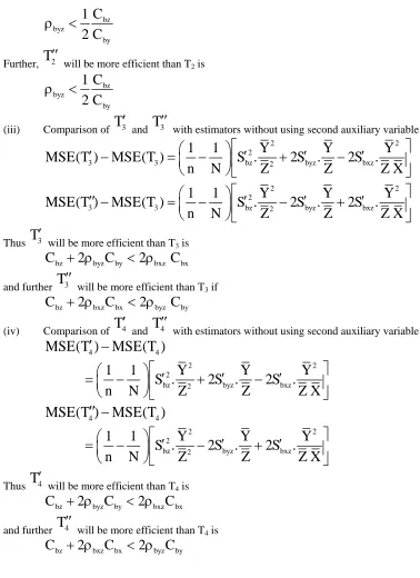
(iii) Comparison of

T

3

′

_and

T

3

′′

_{with estimators without using second auxiliary variable z.}

2 2

2

3 3 bz 2 byz bxz

1

1

Y

Y

Y

MSE(T ) MSE(T )

S .

2S .

2S .

n

N

Z

Z

Z X









′

−

=

_

−

_{ }

′

+

′

−

′

_



_{ }



2 2

2

3 3 bz 2 byz bxz

1

1

Y

Y

Y

MSE(T ) MSE(T )

S .

2S .

2S .

n

N

Z

Z

Z X









′′

−

=

_

−

_{ }

′

−

′

+

′

_



_{ }



Thus

T

3

′

_{will be more efficient than T}

3 is

bz byz by bxz bx

C

+ ρ

2

C

< ρ

2

C

and further

T

3

′′

_{will be more efficient than T}

3 if

bz bxz bx byz by

C

+ ρ

2

C

< ρ

2

C

(iv) Comparison of

T

4

′

_and

T

4

′′

_{with estimators without using second auxiliary variable z.}

4 4

MSE(T ) MSE(T )

′ −

2 2

2

bz 2 byz bxz

1

1

Y

Y

Y

S .

2S .

2S .

n

N

Z

Z

Z X







_{ ′}

_′

_′

=

_

−

_{ }

+

−

_



_{ }



4 4

MSE(T ) MSE(T )

′′ −

2 2

2

bz 2 byz bxz

1

1

Y

Y

Y

S .

2S .

2S .

n

N

Z

Z

Z X







_{ ′}

_′

_′

=

_

−

_{ }

−

+

_



_{ }



Thus

T

4

′

_{will be more efficient than T}

4 is

bz byz by bxz bx

C

+ ρ

2

C

< ρ

2

C

and further

T

4

′′

_{will be more efficient than T}

4 is

bz bxz bx byz by

C

+ ρ

2

C

< ρ

2

C

V. NUMERICAL STUDY

This population is MU 284 population available in Sarndal, Swensson and Wretman (1992, P- 660, Appendix –C). It consists of 284 Municipalities (ssu) divided into 15 clusters (fsu) with three variables i.e. Revenues from the 1985 municipal taxation as y, 1975 population as x and 1985 population as z. For comparison of mean square error of T0, T1, T2, T3, T4,

T5,. 1 1 2 2 3 3 4 4

T , T , T , T , T , T , T , T

′ ′′ ′ ′′ ′ ′′ ′ ′′

, 1

ˆ

Y

, C

ˆ

Y

[image:6.612.33.411.54.574.2]

we consider two-stage sampling with n = 5 and mi (i = 1, 2, … 15) are assumed to be 2, 2, 2, 2, 2, 2, 3, 2, 3, 2, 2, 3, 2, 3, 2.

Table 1: Comparison of Mean Square Errors (MSE)

T0 35564.168

1

T

′

12139.82

1

T

′′

8124.30

T1 548.375

2

T

′

45093.81

2

T

′′

438.25

T2 13182.34

3

T

′

34302.88

3

T

′′

30287.36

T3 22711.44

4

T

′

11921.06

4

T

′′

7905.54

T4 329.61

Remarks

From the above numerical illustration,

(i) MSE(T4) < MSE(T1) < MSE(T2) < MSE(T3) < MSE(T0) (ii) MSE(T'4) < MSE(T'1) < MSE(T'3) < MSE(T'2)

(iii) MSE(T''2) < MSE(T''4) < MSE(T''1) < MSE(T''3)

Also, T4 is more efficient than all other estimators under comparison. However, the results obtained through numerical illustration is not conclusive because of limitations of data. Moreover, the efficiency of an estimator using second auxiliary variable z at the primary stage depends on the correlation structure between x and z at the primary stage.

VI. SUMMARY AND CONCLUSION

Using first stage information on second auxiliary variable z, a number of ratio type estimators in two-stage sampling have been suggested and it is seen that the proposed estimators are more efficient than the competitive estimators using auxiliary information on x only under certain sufficient conditions.

REFERENCES

[1] Chand, L. (1975). Some ratio type estimators based on two or more auxiliary variables. Ph. D thesis submitted to IOWA State University, Ames, IOWA, USA. [2] Sukhatme, P.V. and Sukhatme, B.V. (1970). Sampling theory of surveys with applications. second edition, Asia Publishing House, Bombay, India.

[3] Swain, A.K.P.C. (1970). A note on the use of multiple auxiliary variables in sample surveys. Trabajos de Estadistica, 21, 135-141. [4] Murthy, M.N. (1967). Sampling Theory and Methods. Statistical Publishing Society, Calcutta, India.

[5] Srivastava, S.K., (1967). An estimator using auxiliary information in sample surveys, cal. Stat. Assoc. Bull., 16, 121-132.

[6] Panda, P. (1998). Some strategies in two-stage sampling using auxiliary information. Unpublished Ph.D. Dissertation, Utkal University, Odisha, India.

AUTHORS

First Author – A.K.P.C. Swain, Former Professor of Statistics, Utkal University, Bhubaneswar 751004, Odisha, India.