A new image segmentation algorithm based on SRG and ACM

Journal of Chemical and Pharmaceutical Research, 2014, 6(8):227-237

Research Article

_{CODEN(USA) : JCPRC5}

ISSN : 0975-7384

A new image segmentation algorithm based on SRG and ACM

Bo Cai

1,2

1

Southwest University of Science & Technology, Mianyang Sichuan, China

2

China Academy of Engineering Physics, Mianyang, Sichuan, China

_____________________________________________________________________________________________

ABSTRACT

This paper proposes a new region-based active contour model for image segmentation, which is robust to background difference and intensity non-uniformity. The proposed model is different from other general region-based models: Firstly, SRG model is added to the segmentation as a pre-segment process; Secondly, considering of intensity and gradient variation of the different input images and regions, we using the contour of pre-segmented region’s contour as the iteration source, it make the evolution be robust on condition of the noise and intensity non-uniformity; In addition, the gradient information and the pre-segmented edge information are combined to segment the region, this process enhances the ability of capturing the complex topological structures and making the edge more accurate and stable. Experiments on the natural images demonstrated the desired segmentation performance of our proposed model for the image with intensity non-uniformity.

Keywords: Image segmentation, Active contour model (ACM), Seed region-growing (SRG), Active region, Image

gradient.

_____________________________________________________________________________________________

INTRODUCTION

The aim of image segmentation is to divide an image into different categories based on features, such as intensity, color, histogram or context, where each pixel in the image should belong to one class and only one class. It is an essential issue since it is the first step for image understanding and any other, such as feature extraction, recognition and matching, heavily depends on these results. During the last few decades, many segmentation methods have been extensively proposed in the literature. Seeded region growing(SRG) model is a hybrid method proposed by R. Adams and L. Bischof [1]. This algorithm is robust to the large variety of images because the characteristics of rapid and free to tune the parameters. However, the selection of the initial seeds influences the segmentation results very much. How to assign the initial seeds and threshold becomes the major topic in SRG. Chung-Chia Kang etc.[2] using the fuzzy distance to determine the difference between the pixel and region in the consequent region growing and the difference between two regions in the region merging. Guoying Zhang etc.[3] use the Seed Region and Boundary Growing (SRBG) method to segments each bubble separately instead of operating on the whole image. All the SRG and SRBG model are all for the purpose of finding out the exact region of images according to the inner and outer information of the segmented image. But, when the image is complicated and the region gray of the image is similar to the background, the segmentation process become more difficult to realize.

Secondly, they are less sensitive to the location of the initial contour. One of the most popular models is the Mumford–Shah’s model [5], which approximates an image by using a piecewise smooth function with a length penalizing term. Extended from this model, the Chan–Vese [6] model approximates an image by two-phase piecewise constant function. The energy function of the CV model is minimized via the gradient descent equation with respect to the level set function. To represent multiple regions, the authors in [6] proposed a piecewise constant (PC) model based on the CV model by using a multiphase level set formulation. However, this is not always the case when it comes to the background complicated images. For practical application, many works [4, 7, 8] have been reported based on Mumford–Shah function.

Commonly, the natural images have many regions, and the character of the regions is different from each other. Directly using the ACM based model may cause the segmentation result different from our purpose objects because of the inhomogeneity of the image regions. The SRG model has the ability of finding out the homogeneous regions of the image, and each calculating result of SRG has the similar characterization in gray level and geometric position. In this paper, we’ll use the SRG model to roughly segment the image, and then using the ACM to deal with each result region of SRG. The rest of this paper is organized as follows: In Section 2, we give the review and analysis of ACM model and region-growing model. And then the limitations and results of these models are proposed according to our experiments. The algorithm of active background segmentation using the seeded region growing and ACM is introduced in Section 3. Section 4 is the implementation and experimental results. Section 5 is the summarization of the proposed algorithm.

2. The review of region-growing and active contour model 2.1 Seeded Region-Growing

After Rolf Adams and Leanne Bischof [1] have given the region-growing model, a lot of study has been done based on it. Let

T

be the set of all unallocated pixels that border at least one

A

_iregion after m-times iterations:

1 1

|

( )

n n

i i

i i

T

x

A N x

A

φ

= =





=



∉

≠





U

IU



(1)

where

N x

( )

is the second-order neighborhood (8-neighbours) of pixel

x

. If

N x

( )

are intersect only one labeled region

A

_i, then define the label

i x

( )

∈

{

1, 2,...,

n

}

to be an index such that

N x

( )

I

A

_{i x( )}

=

φ

. If

N x

( )

meet two or more regions, then the difference should be defined to decide which region it should be. Gomez and Gonzalez [9] has given the difference measure function to decide which region the point should belonging to.

[

]

( )

( ,

)

( )

( )

i

i y A x

x A

g x

mean

g y

δ

=

−

_∈ (2)

and then using the measure function to minimize the following function:

( )

{

|

( )

_i

( )

}

i x

=

i N x

I

A

≠ ∧

φ δ

x

(3)

Because of the existence of transitional regions in the images, Frank Y. Shih etc.[10] consider of the

3 3

×

neighborhood of pixel

x

, and calculate the standard deviations of the local image regions.

9

2

1

1

(

)

9

x i

i

x

x

σ

=

=

∑

−

(4)

where

9

1

1

9

i i

x

x

=

=

∑

. Then they use the normalized deviation to define the condition for the seed pixel and apply the

a b c Fig 1 the rough image, edge pixels and inner pixels of the image

In fact, the SRG model is based on the condition that the regions of image are homogeneous in gray scale. But, when we deal with a natural image, the regions may be context regions, transitional regions, or homogeneous regions. If the SRG algorithm has been directly used to the image, the stop condition may be matched at any local regions of the image, and this may causing over-segmentation of the image. For the purpose of avoiding the false stop condition appears in the processing of region growing, we divide the image pixels as region inner pixels and region edge pixels by using the gradient threshold of image as Fig.1 shows. In Fig 1, the threshold is the mean of the total image gradient. Seeing from the result, we may easily found that the segmentation of image is just to divide the edge pixels of the image according to the gray level characterization of the inner pixels. On this condition, the characterization of inner regions and edges may be considered at the same time. Contrast to the single inner character based algorithms or the edge character algorithms, this algorithm using these two characters at the same time, and it may also give the algorithm more standards in decision. In fact, the segmentation of image may be simply defined as the partition of all the edge pixels into the inner pixel classes according to the geometric character and gray level character.

2.2 The review of active contour model and level set based segmentation

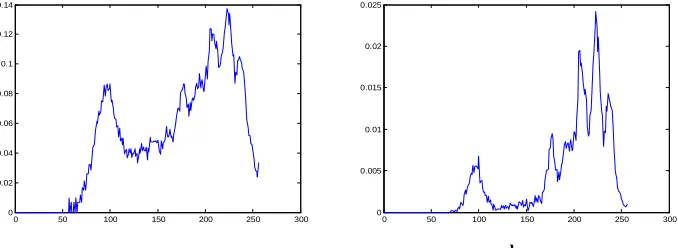
As the above analysis of the image gradient, and the dividing of the pixels, we may simply assume the pixels’ gradient below the mean gradient of the image as the homogeneous regions. Then the only problem is how many regions or classes there are. As to the model of SRG, the main problems are the seeded pixel and the threshold value choosing. Unfortunately, the inhomogeneity of the edge pixels, the difference of gray value between regions may vary from different gray regions. Fig 2 shows the inner gray histogram of the image after dividing according to the image’s mean gradient. From the histogram, we may found one region of the may exist between the other regions, and the edge may be formed by many kinds of gray difference, let alone the transitional and noising of pixels near the edges.

0 50 100 150 200 250 300

0 0.02 0.04 0.06 0.08 0.1 0.12 0.14

0 50 100 150 200 250 300

0 0.005 0.01 0.015 0.02 0.025

[image:3.595.138.477.486.610.2]

a b

Fig 2 The region inner histogram after divided by the gradient (a is divided by mean-gradient and b is divided by 1/2 mean gradient of image)

The ACM based algorithms [13-15] aimed at looking for a particular partition of a given image

I x

( )

into two kinds of regions, one representing the objects to be detected and the other representing the background. For a given image

( )

I x

on the image domain

Ω

, they propose to minimize the energy function:

2 2

1 2 1 1 2 2

( ) ( )

( ,

, )

( ( )

)

( ( )

)

CV

in C out C

E

c c C

=

λ

∫

I x

−

c

dx

+

λ

∫

I x

−

c

dx

(5)

2 2

1 2 1 _{( )} 1 2 _{( )} 2

( ,

, )

( ( )

)

( ( )

)

( )

( ( ))

CV

in C out C

E

c c C

I x

c

dx

I x

c

dx

Length C

Area in C

λ

λ

µ

ν

=

−

+

−

+

+

∫

∫

(6)

Using the level set to represent C the zero level set of a Lipschitz function

φ

( )

x

, and then the energy function may be written as:

2 2

1 2 1 1 2 2

( ,

, )

( ( )

)

( ( ))

( ( )

) (1

( ( )))

( ( ))

( )

( ( ))

CV

E

c c

I x

c

H

x dx

I x

c

H

x

dx

x

x dx

H

x dx

φ

λ

φ

λ

φ

µ δ φ

φ

ν

φ

Ω Ω

Ω Ω

=

−

+

−

−

+

∇

+

∫

∫

∫

∫

(7)

where

H

( )

φ

and

δ φ

( )

are Heaviside function and Dirac function, respectively.

To overcome the difficult caused by intensity in-homogeneity, Li et al. proposed the local binary fitting (LBF) model [16, 17], which utilize the local intensity information to fit the energy function.

For all the center point x in the image domain

Ω

, the energy function is defined as:

2

1 2 1 1

2

2 2

( ,

( ),

( ))

(

)( ( )

( ))

( ( ))

(

)( ( )

( )) (1

( ( )))

LBF

E

C f x

f x

g x

y I y

f x

H

y dy dx

g x

y I y

f x

H

y

dy dx

λ

φ

λ

φ

Ω Ω

Ω Ω





=

_

−

−

_





+

_

−

−

−

_

∫ ∫

∫ ∫

（8）

where

g x

(

−

y

)

is a Gaussian weighted coefficient of the local information. Because of using local region information, specifically local intensity mean, the LBF model is able to provide desirable segmentation results when the image is two phrased. From the analysis of the above models, we found that the seed region-growing model is using the local information much more than the ACM based models, and the ACM models considered more total information than seed region-growing model in image segmentation. Combining of these two kinds of models, may leads to the better results in image segmentation.

3. The proposed algorithm based on SRG and ACM/CV models

Threshold is a pixel classification process to identify the pixels of a given image into two classes: those pertaining to objects and those pertaining to background. Given an input image

f

, the threshold segmentation is defined as:

[image:4.595.135.478.504.615.2]

a b c

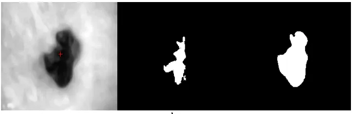
Fig 3 The SRG based region growing result (a. the seed point of the input image; c. the result with threshold 10; d. the result with threshold 40)

1, ( , )

( , )

0, ( , )

f x y

T

g x y

f x y

T

≥



=



<



(9)

distribution of the image gray levels. From Fig.1(a) and Fig.2(b), we roughly divide the image’s gray level into 5 classes according to the Gaussian distribution characterization. The simplest way of dividing the image gray is to divide the histogram from the lower gray level to the higher gray level or on the contrary.

0 50 100 150 200 250 300

0 50 100 150 200 250 300 350 400

[image:5.595.119.509.120.243.2]

(a) (b) (c)

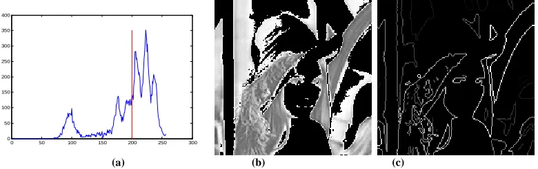
Fig 4 a is the histogram and the extraction of the first two-phase gray scale; b is the result of the extracted image; c is the LGIF segment result of the image lower gray parts

According to the above analysis of the two-phase image extraction, we give the experiment result in Fig 4(c). From the segmented result, we may found there are some wrong regions been segmented. The following step is the extraction of the reasonable regions. Given a gray scale image, a gradient is represented by its horizontal

G

_x and vertical

G

_y components. Given a gray level image

I

_{M N×} , we take the magnitude of the gradient as:

(

)

(

)

2

(

)

2

,

x

,

y

,

,

1, 2,

, N;

1, 2,

,

G m n

=

G

m n

+

G

m n

n

=

K

m

=

K

M

(10)

For the purpose of estimating the stability of the regions after each segmenting, we use the coincidence degree between the edge of threshold segmented region and the gradient as the stability of the segment result. If the stability is higher, the region would be extracted from the image and the histogram, before the next segmentation. The calculation of the normalized stability may be simply defined as:

,

1

( , )

( , )

(

)

i

i i

i

m n

Stab

G m n

Edge

m n

Count Edge

_{Ω ∈Ω} Ω

=

∑

×

(11)

where

Ω

_iis the ith region of present threshold segmented results;

G m n

( , )

is the magnitude of the gradient;

(

)

i

Count Edge

_Ω is the pixel number of

Ω

_i’s edge; the

( , )

i

Edge

_Ω

m n

is defined as a binary function, when the

point

(

m n

,

)

is on the edge of

Ω

_i, the value is 1, otherwise 0. Fig.4(d) shows the stability of the segmented regions.

(

)

( )

0,

,

( , )

1,

i

i

if m n

inner

Edge

m n

otherwise

Ω

∈

Ω



=





(12)

0 20 40 60 80 100 120 140 160 180 200 0

[image:6.595.101.514.332.578.2]

0.05 0.1 0.15 0.2 0.25 0.3 0.35

Fig 5 The extracted regions of the lower and upper two-phase images (a is the lower gray range, b is the upper gray range, c is the sum edges of lower and upper sides, d is the normalized gradient of the region edge)

4. The design and realization of active region based model

In this part, the process of image segmentation will be presented, according to what have been stated in part 3. The process may be divided into three steps:

(1) For the purpose of avoiding the noise, the image should be smoothed using the gauss kernel function; (2) Choosing the seed pixels;

(3) Considering the histogram of the image and finding the threshold of SRG, and pre-segment the key region from the processing image;

(4) Using the adjusted ACM model to divide the local region into two main regions. Fig.4 is the main process of segmentation:

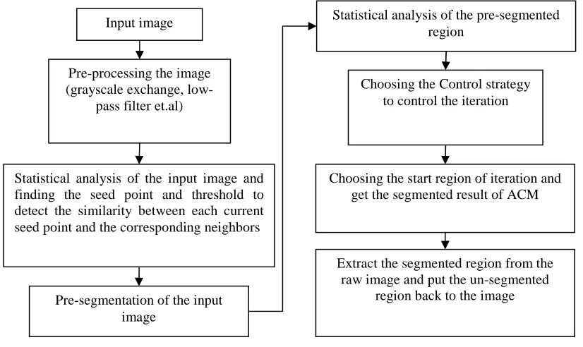
Fig 6 the main process of segmentation

4.1 pre-processing of the input image

Often, image noise and blurring cause errors in region-growing leading to the segmentation difference from different backgrounds. The initial seed pixel should have high similarity to its neighbors [18] and not on the edge or detailed region. Therefore, the criterion of the initial seeds selection in [2] is that

If

min(

NCE

_{i j,}

,

S

_{i j,}

)

≥

T

_{i j,} , then

x

_{i j,} is a seed, (13)

where

T

_{i j,} is a threshold determined by a fuzzy rule base to avoid getting the edge point of the image.

S

_{i j,} is a fuzzy similarity between each current pixel

x

_{i j,} and the corresponding neighbors.

x n

_n

,

=

1, 2,..., 9

and

x

_meanare nine pixels in the sliding window whose center is

x

_{i j,} and the mean of their vector, respectively.

w

_s is set to 0.4 in the common case.

Input image

Pre-processing the image (grayscale exchange,

low-pass filter et.al)

Statistical analysis of the input image and finding the seed point and threshold to detect the similarity between each current seed point and the corresponding neighbors

Pre-segmentation of the input image

Statistical analysis of the pre-segmented region

Choosing the Control strategy to control the iteration

Choosing the start region of iteration and get the segmented result of ACM

Extract the segmented region from the raw image and put the un-segmented

9

,

1

1

1

min

,1

9

n mean i j n s

x

x

S

w

=



₋



= −









∑

(14)

The seed choosing is also an important part in our model, so we choosing the way as [2] the standard to determine whether the point is the seed pixel. As to the threshold

T

_{i j,} of equation (13), we choose the

5 5

×

window. As to the smooth kernel, for the purpose of avoiding being influenced by the noise of the image, we choose the average kernel as ACM model does.

4.2 Grayscale threshold-choosing and region-growing

In this step, the seeded regions grow pixel by pixel. [2] using the pixel label way to detecting the region, and dividing the neighbors of one pixel into three cases. After the pixel is labeled to one region, they remove it from

H

and add the unlabeled neighbors into

H

. Thus update the region mean value

R

_m

,

m

=

1, 2, 3,...,

M

. The region growing step works iteratively until H is empty, i.e. all pixels in the image are labeled. Because of this region growing ways need to adjust the mean value

R

_min the step of segmentation, our purpose in region growing is to get the rough region of what we want to segment, so we need only to take a seed pixel and growing it. The step of growing process may be simply divided into four steps:

(1) Choosing the seed pixel of region growing;

(2) Choosing the threshold of this region growing according to the histogram of the input image; (3) Finding the similar pixels of the image within the threshold and its adjacent;

(4) Extracting the region from the image.

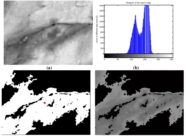
0 200 400 600 800 1000 1200 1400 1600 1800

Histgram of the input image

gray level c o u n t o f d if fe re n t g ra y l e v e l (n )

0 50 100 150 200 250

(a) (b)

[image:7.595.144.469.364.602.2]

(c) (d)

Fig 7 the main process of segmentation using region-growing, (a) rough image; (b) the rough image’s histogram; (c)the seed point and segmented region in binary image; (d) the region’s rough grayscale of image

We considering the histogram of the input image and choosing the threshold as about 20% grayscale range of the image as the threshold. The input image for example Fig.5 (a), the grayscale range

[

90, 177

]

, seed pixel’s grayscale is 125, and the image total pixels

306 313

×

=

95778

, the point count is (17):

125 125

( )

threshold i threshold

count i

+ = −









where

count i

( )

is the statistic histogram value of the input image. In our experiment we’ve been used the threshold 20, 25, 30 and 35 to testing the segmentation, the result of the segmentation has only about 20% difference in result region area. Fig.5 shows the process of seed region growing segmentation when taking the threshold 20 with absolute image gradient.

4.3 The process of segmented region and iteration based on ACM

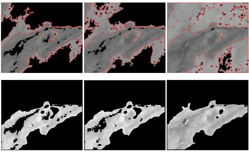
In most study of image process, the image and region are considered as matrix, when the region is not a matrix region, the difference of the background and the segmented region may causing much contour in the processing. The first step of our model is to deal with the edge of the segmented region and cancel its influence in the iteration of ACM. In the iteration of ACM, it using the forward and backward gradient to calculate the contour of the image, for the purpose of making the iteration converge to the inner region of the pre-segmented area, we calculate the inner contour and control calculating of the parameters according to the inner of the pre-segmented region.

[image:8.595.149.465.227.345.2]

(c) (d)

Fig 8 The contour of the segmented region: (a) the segmented region and edge contour; (b) the inner contour of the segmented region

After dealing with the contour of the segmented region, we use the energy function as Eq.8 to calculate the minimizing energy of the segmented region. The first column of Fig.7 is the segmented results of the input image. In the experimentation we choose the threshold of grayscale as 20, 25 and 30 to pre-segment using SRG, then using the parameters for the ACM model as:

1 2

1

λ λ

=

=

,

µ

=

1

,

v

=

0.01 255 255

×

×

,

∆ =

t

0.1

,

itertimes

=

100

.

In our experiment, we are aimed at segment the area which contains the seed pixel, after the iteration stop, we must get the segmented area from the image according to the contour and edge of the pre-segmented region as 4.1 stated.

[image:8.595.102.509.488.737.2]

[image:9.595.148.464.117.375.2]

Fig 10 is the result of the rough image using ACM, LBF and LGIF. Comparing the result of this three model’s result to the result of Fig 9, we may found that the results of ACM and LGIF are similar to the result of our model, and the LBF result is very different to others.

(a) (b)

(c) (d)

Fig 10 the result of ACM, LBF and LGIF: (a) input image; (b) ACM result of 1000 times iteration; (c) LBF 1000 times iteration; (d) LGIF 400 times iteration

DISCUSSION

In this section, we will give the discussion of the experimental results of the proposed algorithm. For the purpose of comparing the stability of this model to the ACM, LBF and LGIF, we choose the segmented region’s difference as the standard of the stability. When the input image is large, the time consuming of iteration becomes very long. The calculation of the difference is defined as:

( )

(

1)

( )

diff i

=

area i

+ −

area i

(16)

where

area i

( )

and

area i

(

+

1)

is

i i

,

+

1

times iteration result of the region where the contour and edge enclosed and the seed pixel is in the region at the same time. Fig 11 shows the convergence processing of ACM, LBF and LGIF.

0 50 100 150 200 250 300 350 400 0

1 2 3 4 5 6 7 8 9 10x 10

4

1-400 times iteration

c

o

u

n

t

o

f

th

e

r

e

g

io

n

c

o

n

ta

in

s

t

h

e

s

e

e

d

p

ix

e

l ←_← LGIF iterative LCV iterative

← LBF iterative

the region area contain the seed pixel

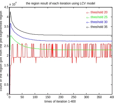
[image:9.595.206.400.573.728.2]

Fig 11 and Fig 12 show the convergence processing of our model, for the purpose of comparing to the above mentioned models (LCV, LBF, and LGIF), we choose the threshold as 20, 25, 30 and 35 to iterate 400 times.

0 50 100 150 200 250 300 350 400 0 0.5 1 1.5 2 2.5 3 3.5 4 4.5x 10

4 _{the region result of each iteration using LCV model}

times of iteration 1-400

c o u n t o f th e r e g io n g o tt f ro m t h e p re -s e g m e n te d r e g io

n _← threshold 20

← threshold 25

← threshold 30

← threshold 35

Fig 12 the process of LGIF after the segmentation of SRG

Comparing these two kinds of segment process and result, when the threshold is 20, 25, 30 and 35, the regions’ much of the contour is in critical threshold. When the threshold reached to 40 and 45, the iteration converged quickly, and the region difference has only about 10% in pixel counts.

CONCLUSION

In this paper, we proposed a new region-based active contour model for image segmentation, which is robust to background difference and intensity non-uniformity. The proposed model is different from other general region-based models in three ways. Firstly, SRG model is added to the segmentation as a pre-segment process; Secondly, considering of intensity variation of the different input image we using the contour of pre-segmented region’s contour as the iteration source, it make the evolution be robust to the noise and intensity non-uniformity; In addition, the gradient information and the pre-segmented edge information are combined to segment the region, this process enhances the curve’s ability of capturing the complex topological structures and making the edge more accurate and stable. The experiments on the natural images demonstrated the desired segmentation performance of our proposed model for the image with intensity non-uniformity.

Acknowledgements

The authors thank the anonymous reviewers for their many valuable comments and suggestions that helped to improve both the technical content and the presentation quality of this paper.

REFERENCES

[1] R. Adams and L. Bischof, Pattern Analysis and Machine Intelligence, 1994, vol. 16, pp. 641-647.

[2] C.-C. Kang, W.-J. Wang, and C.-H. Kang, AEU - International Journal of Electronics and Communications,

2012, vol. 66, pp. 767-771.

[3] Z. Guoying, Z. Hong, and X. Ning, Mining Science and Technology (China), 2011, vol. 21, pp. 239-242. [4] M. Lee, W. Cho, S. Kim, S. Park, and J. H. Kim, Comput Biol Med, May 2012, vol. 42, pp. 523-37. [5] S. Shah and J. K. Aggarwal, Pattern Recognition, November 1996, vol. 29, pp. 1775-1788.

[6] T. F. Chan and L. A. Vese, Image Processing, IEEE Transactions on 2001, vol. 10, pp. 266-277. [7] Y. Zou, H. Liu, and Q. Zhang, Digital Signal Processing, 2012.

[8] X. Jiang, R. Zhang, and S. Nie, Physics Procedia, 2012, vol. 33, pp. 840-845.

[9] O. G´omez, J. u. A. Gonz´alez, and E. F. Morales, Computer Science, 2007, vol. 4756, pp. 192-201. [10] F. Y. Shih and S. Cheng, Image and Vision Computing, 2005, vol. 23, pp. 877-886.

[11] L. S. Hibbard, Med Image Anal, Sep 2004, vol. 8, pp. 233-44.

[12] G. C. Lin, W. J. Wang, C. C. Kang, and C. M. Wang, Magn Reson Imaging, Feb 2012, vol. 30, pp. 230-46. [13] Q. Ge, L. Xiao, J. Zhang, and Z. H. Wei, Pattern Recognition Letters, 2012, vol. 33, pp. 1549-1557. [14] Q. Ge, L. Xiao, H. Huang, and Z. H. Wei, Digital Signal Processing, 2012, pp. 238-243.

[image:10.595.206.401.110.290.2]

[16] C. Li, C.-Y. Kao, J. C. Gore, and Z. Ding, Image Processing, IEEE Transactions on 2008, vol. 17, pp. 1940-1949.

[17] K. Zhang, H. Song, and L. Zhang, Pattern Recognition, 2010, vol. 43, pp. 1199-1206.