142
A NOVEL BINOMIAL TREE APPROACH TO CALCULATE
COLLATERAL AMOUNT FOR AN OPTION WITH CREDIT
RISK
SASTRY KR JAMMALAMADAKA1. KVNM RAMESH2, JVR MURTHY2
Department of Electronics and Computer Engineering, Computer Science and Engineering KL University1, Jawaharlal Nehru Technological University2
Vaddeswaram, Guntur district, Andhra Pradesh, India 522502 Kakinda, Andhra Pradesh, India 533503
E-mail: [email protected], [email protected], [email protected]
Abstract: Options traded over-the-counter are associated with credit risk and are called vulnerable options.
Collateral can be taken to mitigate the credit risk. However the amount of collateral should be such that it shouldn’t take into account the almost not plausible states of the underlying which when considered increases the required collateral amount. This paper proposes a methodology to calculate the optimum collateral amount that is required from the seller of a vulnerable option. The calculated collateral makes the vulnerable option as risky as the exchange traded option. The algorithm to calculate the optimum collateral uses the novel binomial decision tree built without any assumption on the underlying distribution. The study reveals that the price of a vulnerable option converges to an exchange traded option as the collateral amount reaches a certain optimum value. The proposed methodology will be of interest to the option seller so that the excess collateral above the optimum collateral can be used for some other purposes.
Keywords: Binomial Tree, Credit Risk, Collateral Amount, Option pricing, Venerable options, Margin Computation
1 INTRODUCTION
Derivatives are financial instruments that are used to transfer the risk in an underlying to counterparty. One such derivative is an option which gives the buyer the right but not the obligation to exercise the same. However the counterparty which sells the option has to obey the option contract if it turns in-the-money. For entering into an option transaction, the option buyer has to pay certain premium for transferring the risk in the underlying to the option seller. If the option is exchange traded, the risk associated with it is considered free of credit risk, as the probability of default of an exchange is almost zero. In case of options traded over-the-counter (OTC) which are called vulnerable options a considerable amount of credit risk is associated with the option seller. Hence the option buyer can demand collateral to mitigate the credit risk associated with the vulnerable option.
Many works have been presented [4][6][7][8][10]in the literature which focus on pricing of vulnerable European options. Binomial trees [11] [14] can be used to price both European and American style vulnerable options. Although these methods, price vulnerable options for a
given collateral amount they do not give an estimate on the optimum collateral amount at which the vulnerable option is as risky as an exchange-traded option. It has been found that [8] the collateral calculated is constant irrespective of strike price and covers almost implausible states that the underlying can take.
In this work, the problem of calculating the optimal collateral amount that makes the vulnerable option as risky as an exchange-traded option is presented. The collateral calculation algorithm overcomes the constant collateral amount for all strikes as in [8] and considers only the plausible states at a given percentile.
The collateral amount calculated using the pricing formula proposed in [8] is compared with the collateral amount calculated based on the algorithm presented in this paper, which prices the vulnerable based on a binomial tree proposed in [11].
143 option and discusses the algorithm to calculate optimum collateral. The convergence of the collateral amount and the sensitivity of the price of vulnerable option are modelled and presented in this paper. A comparative study of the collateral amounts calculated using pricing formula proposed in [8] and with the algorithm discussed in section 4 using the binomial tree proposed in [11] is presented in section 4.3. Section 5 concludes and gives a direction to future work.
2 LITERATURE SURVEY
The breakthrough in pricing of options is the famous Black-Scholes model [1], which prices European options on an underlying following Brownian motion. While considering credit risk, derivatives are viewed as compound options on the assets underlying the financial securities as in the case of Merton [12] [13], Black and Cox [2], Ho and Singer [5], Chance [3] and Kim, Rama Swamy and Sundaresan [9]. Johnson and Stulz [8] proposed the valuation model concerning the issue of counterparty credit risk, assuming that the option itself is the only liability of the option writer, and the default occurs when the option writer's collateral assets cannot afford the promised payment in the option contract. They also introduced the term “vulnerable option” for an option that contains counterparty credit risk. Their approach is an extension of the corporate bond model presented by Merton [12]. Hull and White [7] extended the credit risk model of Johnson and Stulz [8] to bond pricing models related to the first passage time. Jarrow & Turnbull [7] also considered early default in studying the effect of default risk on fixed income and other options. Considering the correlation between the underlying asset price and the assets value of the option writer, they assumed that an option writer defaults on its obligations when an exogenously specified boundary is reached by the assets value of the option writer. Klein [7] further modified Johnson and Stulz [8] assumption by allowing the option writer to have other liabilities of equal priority payment under the option. Klein [10] developed close-form solutions for Black-Scholes options subject to credit risk of the option writer's default event. Cochrane and Saá-Requejo [4] developed a methodology to price vulnerable options with stochastic and deterministic interest rates in an incomplete market. They have proposed a methodology that can price vulnerable options in incomplete markets considering
liquidity risk into account. Hui, Lo and Ku [4] developed a valuation model of European options incorporating a stochastic default barrier extending the constant default barrier proposed in the Hull-White model.
Most of the literature is focused on pricing of vulnerable European options under the assumption of lognormal distribution of stock prices.
The methods existing in the literature, price a vulnerable option given a collateral amount and theoretically require infinite collateral amount to make the option credit risk free. Therefore calculation of optimum collateral amount at which the credit risk is zero is a problem of interest.
While using the methodology proposed in [8] for vulnerable option pricing when the collateral is cash, it is observed that the collateral amount is constant irrespective of strike and implausible prices of the underlying are considered for collateral calculation.
KVNM Ramesh et.al [11] proposed a methodology to build a binomial tree that is independent of underlying distribution of the stock prices. Binomial tree distribution shown in [11] to found be more efficient compared to lognormal distribution of stock prices for estimating the stock prices.
In this work, we used the methodology discussed in [11] to generate the binomial tree of stock prices. The tree is used to compute the option prices of both vulnerable and non-vulnerable option. The tree can be used to price both European and American vulnerable options. We propose an algorithm that computes the optimum collateral amount at which the vulnerable option is credit risk free. The collateral calculation algorithm can also be used for both European and American vulnerable options.
Experiments were carried, keeping the risk coverage as constant and observed that the collateral varies with the strike.
144
3 BINOMIAL TREE BUILDING
The underlying stock process is assumed to follow a binomial process where the magnitudes of the upward and downward movements are governed by the risk neutral pricing principles. While building the binomial tree the stock price at time t is denoted St, and the next period’s stock
price St+h may take one of two possible values:
u St (an up move) w / prob pu St+h = (1)
d St (a down move) w / prob pd
where
u- Upward multiplier d- Downward multiplier q- Probability of up move h- Length of time step
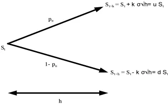
This can be represented in figure [1] where the magnitude of up move and down move is also represented.
St
St+h = St + k σ√h= u St
St+h= St - k σ√h= d St
pu
1- pu
[image:3.595.110.282.398.506.2]h
Figure 1: Binomial Tree for one step
Under risk neutral pricing, the price of the underlying should grow at a risk free rate ”r”. Hence the expected value at maturity should follow equation (2).
pu * u St + (1- pu )d St = St * erh
(2)
pu = (erh – d)/(u-d)
(3)
u= 1 + k σ√h/ St
(4)
d= 1 - k σ√h/ St
(5)
Where
k – is the confidence factor used in building the tree
σ- Absolute volatility of the underlying daily returns
In order to make the tree recombining with constant probabilities of upward and downward movements the value of u and d are chosen as shown in equation(6) and (7).
u= 1 + k σ√h/ S0
(6)
d= 1 - k σ√h/ S0
(7)
The advantage with recombining trees is that the numbers of computations are decreased compared to non-recombining tree.
4 VULNERABLE OPTION PRICING
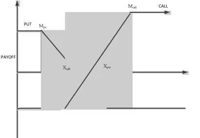
The payoff of a vulnerable option is dependent on whether the collateral amount pledged by the option writer can afford to pay the promised payment. Assuming the collateral amount is “M” the payoff of a vulnerable option is given by equation (9) which is diagrammatically represented in figure (2).
Payoff = Minimum (M, Maximum [(ST – X), 0]
for call option (9)
Minimum (M, Maximum [(X- ST), 0]) for put
option Where
M - Risk free collateral amount at maturity
ST – Underlying Price at Maturity
X – Strike price of the option
The payoffs at maturity are discounted by backward valuation using the tree built as discussed in section 1. The discounted value at node zero gives the premium of the vulnerable option. For an American style option the probability of early execution is also considered when the underlying price at step s satisfies the condition shown in equation (10).
M ≤ Ss –X
145 Where
Ss – Underlying price at step
Step “s” will be a part of the tree. In figure 1 only one step is shown. The same can be extended to “n” number of steps within which “s” is one of the steps. The terminal values at each step are multiplied with “u” and “d” as given in equations (4) and (5) to get the values at the next step.
Algorithm to calculate minimum collateral
Though the vulnerable option is traded over-the-counter (OTC), the credit risk associated with the option can be mitigated by pledging a minimum amount of collateral so that the vulnerable option is as good as the exchange traded option. In this section we describe the algorithm to calculate the minimum collateral amount using the tree built in section 1.
PAYOFF PUT
CALL
ST
Xcall Xput
Mpu t
Mcall
Figure 2 Payoff for a Vulnerable Put and Call options
Algorithm
1. Start
2. The range of M lies between (0, 100*S0 )
where S0 is the spot price of the
underlying stock.
3. Let Mlow = 0 and Mhigh = 100*S0, Δold =
100000000
4. Let Pe be the value of exchange traded
option using the binomial tree of section 1.
5. Let Pv be the value of the vulnerable
option with the value of M = (Mlow +
Mhigh)/2
6. Compute Δ = Pv – Pe
7. If | |Δold|- |Δ| | < µ then go to step 16
8. Else
9. Δold = Δ; Mprev = M
10. End if
11. If Δ < -1 Mlow = M
12. Else 13. Mhigh = M
14. End if 15. Go to step 5
16. The value in Mprev gives the Minimum
collateral required. 17. End
4.1 Sensitivity of the Collateral and Vulnerable Option Price to Model Parameters
The collateral requirement increases with the strike price of the put option and decreases with the strike price of the call option. However for a given option, it can be observed from figure [3] that the price of a vulnerable option converges to the price of the riskless option as the collateral amount increases also the change in Δ with the change in value of collateral (M) after certain value of M is almost constant. From this it can be inferred that if the value of Δ is very small then the amount of collateral required is much higher to cover even the least possible payoffs which is undesirable from the view of option writer.
The inflection point at which the price of the vulnerable option converges almost to the price of the riskless option represent the minimum collateral required to cover the option position for credit risk.
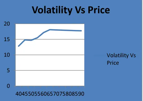
The price of a vulnerable option is compared to a vanilla option which is a normal call or put option that has standardized terms and no special or unusual features and generally traded on an exchange. Figure [4] explains that the price of a vulnerable option need not always increase with maturity as opposed to the price of a plain vanilla option whose price increases with maturity. From figure [5] it can be observed that the price of the vulnerable option may decrease with increase in volatility as opposed to the price of a vanilla option whose price increases with volatility.
4.2 Comparative Analysis
[image:4.595.96.300.368.509.2]146 Considering a call option the formula to price a vulnerable option as given in [8] is given in equation (11) with the option price calculated using the Black-Scholes model [1].
c(S(t), M, X, T) = c(S(t), X, T) - c(S(t), M, T) (11)
where
c(S(t), M, X, T) is price of vulnerable option c(S(t), X, T) is price of uncapped option
c(S(t), M, T) is price of option with payoff capped to M
X is the strike price of option T is the maturity of option S(t) is the value of the underlying
From the equation (11) the value of collateral M that is required to cover 100% of the risk is equal to the strike price (Mmax) at which the price of the
call option is zero so that the value of the vulnerable option is same as that of exchange traded option.
The disadvantage with this approach is the value of the collateral does not change with the strike price. However as the strike price increases and the probability that the option turns in-the-money decreases.
Therefore, the collateral amount required covering that payoff should be less than Mmax. To
consider this effect the collateral calculation algorithm presented above considers vulnerable call option as a capped call option whose cap is considered as the required collateral. The cap is varied such that the price of the equivalent uncapped option is same as that of the capped option.
Table I shows the value of collateral amount computed using the algorithm given in section 4.
Table II shows the collateral calculations following equation (11). Both the computations are done with underlying price at 5000, one month maturity, 10% risk free rate and 30% volatility.
Table I: Collateral calculated at various strike prices S tr ik e P ri ce C o llat er al B y p ro p o se d m eth o d C o v er ed U n d er ly in g p rice at matu ri ty B y p ro p o se d m eth o d R is k C o v er ed b y c o llater al cal cu late d b y p ro p o sed m eth o d
1000 6000 7000 99.9900%
2000 5000 7000 99.9900%
3000 4000 7000 99.9900%
4000 3000 7000 99.9900%
5000 2000 7000 99.9900%
6000 1000 7000 99.9900%
7000 500 7500 99.9995%
8000 100 8100 100.0000%
The strike price at which the value of the call option becomes zero is 7700. From Tables I and II it can be seen that the methodology proposed in II for collateral calculation considers the most implausible events for the underlying prices at maturity and hence reports excess collateral. Also the collaterals for deep-in-the money options calculated using the proposed methodology approaches the collateral calculated following equation (11). Hence the proposed methodology will be of interest to the option sellers as the collateral requirement is not flat and considers plausible events at 99.99% confidence.
Table II: Collateral calculated at various strike prices S tr ik e P ri ce C o ll ater al F o ll o wi n g e q u a ti o n (1 1 ) C o v er ed U n d er ly in g p rice at m atu ri ty F o ll o wi n g e q u a ti o n (1 1 ) R is k C o v er ed b y co llat er al cal c u lat e d F o ll o wi n g e q u a ti o n (1 1 )
1000 7700 08700 100%
2000 7700 97000 100%
3000 7700 10700 100%
4000 7700 11700 100%
5000 7700 12700 100%
6000 7700 13700 100%
7000 7700 14750 100%
8000 7700 15810 100%
147 The proposed work has the following assumptions and limitations:
1. Markets for traded assets are perfect with no taxes and transaction costs, no limit on short sales with all investors as price takers
2. There exists unlimited borrowing at constant interest rate per unit time 3. The underlying can’t take negative
values.
4. Markets are complete so that it is possible to construct a portfolio that pays nothing until maturity and maturity value at maturity and a portfolio that pays nothing until maturity and collateral amount at maturity.
5. The collateral is in the form of cash in the same currency as the underlying. 6. It is assumed that there exists an
equivalent exchange traded option for the corresponding vulnerable option.
5 CONCLUSIONS AND FUTURE WORK
In this work we observed that the collateral requirement for the vulnerable call option, increase with decrease in strike price. The collateral calculated using the proposed algorithm approaches the collateral calculated using [8] for deep-in-the money call options. As the strike price of the call option increases, the collateral amount decreases for the same risk coverage. The proposed algorithm will be of interest to the option seller as the collateral decreases for strikes around the current underlying price. The work can be extended to vulnerable options with risky collaterals.
Figure 3 Collateral Vs Difference between Riskless and Vulnerable Option
Figure 4 Maturity Vs Price of the vulnerable option
Figure 5 Volatility Vs Price of the vulnerable option
REFERENCES
[1]. Black F., Scholes M., “The pricing of options and corporate liabilities. Journal of political economy”, 81 pp. 637-654, 1973. [2]. Black F., and J. Cox, Valuing Corporate
Securities: Some effects of bond indenture provisions, Journal Of Finance, 1976, 31, 351-367.
[3]. Chance, D; “Default risk and the duration of Zero coupon bonds, Journal of Financ, 1990, 45, 265-274.
[4]. C.H.Hui, C.F.Lo and K.C.Ku., “Pricing vulnerable European options with stochastic default barriers”, IMA Journal of Management Mathematics, 2007
[5]. Ho. T, and R. Singer “Bond indenture provisions and the risk of corporate debt,
0 20 40 60 80 100 120 140
1
0
0
4
0
0
7
0
0
1
0
0
0
1
3
0
0
1
6
0
0
1
9
0
0
Collateral Vs Delta
Collateral Vs Price
0 5 10 15 20 25 30
0.5 1 2 3 4 5
Maturity Vs Price
Maturity Vs Price
0 5 10 15 20
4045505560657075808590
Volatility Vs Price
[image:6.595.314.539.104.297.2] [image:6.595.312.541.338.500.2]148 Journal of Financial Economics, 1982, 10, 375-406.
[6]. Hull, J. and White, A., The Impact of Default Risk on the Prices of Options and Other Derivative Securities. J. Banking Finance, 1995, 19, 299-322.
[7]. Jarrow, R.A. and S.M. Turnbull, 1995, pricing derivatives on financial securities subject to credit risk, Journal of Finance 50, 53-86.
[8]. Johnson, H. and Stulz, R., The pricing of Options with Default Risk. J. Finance, 1987, 42, 267-280.
[9]. Kim J, K. Ramaswamy, and S. Sundaresan; “Does Default Risk in Coupons affect the valuation of corporate bonds?: A contingent claims model, 1993, Financial Management 117-131.
[10]. Klein, P., “Pricing Black-Scholes options with correlated credit risk. J. Banking Finance”, 1996, 20, 1211-1129.
[11]. K. V. N. M. Ramesh, J. V. R. Murthy, J. K. R. Sastry “Incorporating Implied volatility in Pricing Options using implied Binomial Tree”, 2nd IIMA International Conference on Advanced Data Analysis, Business Analytics and Intelligence, January 8-9, 2011
[12]. Merton, R. C., On the Pricing of Corporate Debt: The Risk Structure of Interest Rates. J. Finance, 1974, 2, 449-470.