Mathematics Theses Department of Mathematics and Statistics
Summer 8-18-2010
Looking in the Crystal Ball: Determinants of Excess Return
Looking in the Crystal Ball: Determinants of Excess Return
Kokou S. Akolly Georgia State University
Follow this and additional works at: https://scholarworks.gsu.edu/math_theses Part of the Mathematics Commons
Recommended Citation Recommended Citation
Akolly, Kokou S., "Looking in the Crystal Ball: Determinants of Excess Return." Thesis, Georgia State University, 2010.
https://scholarworks.gsu.edu/math_theses/87
This Thesis is brought to you for free and open access by the Department of Mathematics and Statistics at ScholarWorks @ Georgia State University. It has been accepted for inclusion in Mathematics Theses by an authorized administrator of ScholarWorks @ Georgia State University. For more information, please contact
KOKOU S.AKOLLY
Under the direction of Dr Jun Han
ABSTRACT
This paper investigates the determinants of excess returns using dividend yields as a proxy in a cross-sectional setting. First, we find that types of industry and the current business cycle are determining factors of returns. Second, our results suggest that dividend yield serves a signaling mechanism indicating “healthiness” of a firm among prospective investors. Third we see that there is a positive relationship between dividend yield and risk, especially in the utility and financial sectors. And finally, using actual excess returns, instead of dividend yield in our model shows that all predictors of dividend yield were also significant predictors of excess returns. This connection between dividend yield and excess returns support our use of dividend yield as a proxy for excess returns.
by
KOKOU S.AKOLLY
A Thesis Submitted in Partial Fulfillment of the Requirements for the Degree of
Master of Science
In the College of Arts and Sciences
Georgia State University
KOKOU S.AKOLLY
Committee Chair: Dr Jun Han
Committee: Dr. Yichuan Zhao
Dr. Gengsheng Qin
Electronic Version Approved:
Office of Graduate Studies
College of Arts and Sciences
Georgia State University
DEDICATION
To my mother, Adjoa Angele Apedjinou.
“Hundreds of dewdrops to greet the dawn, Hundreds of bees in the purple clover, Hundreds of butterflies on the lawn, But only one mother the wide world over.”
TABLE OF CONTENTS
LIST OF TABLES vi
1. Introduction 1
2. Theory and Model 5
2.1 Theory 5
2.2 Model 6
3. Empirical Analysis 7
3.1 Data Description 7
3.2 General Diagnostics 10
3.3 Empirical Analysis (Using Data Subset) 13
3.3.1 Dividends in Different Industrial Sectors 13
3.3.2 Dividends as a Signaling Mechanism 18
3.3.3 Dividends as Compensation for Risk 23
3.3.4 Excess Return model 26
LIST OF TABLES
Table1: Excess Returns: Dividend Yield, Earning Yield, and Payout (Lamont 1996) 3
Table 2: Variables description 8
Table 3: Firms and Industries in AKOLLY30 and DJ30 Indices 9
Table 4: Dividends in different industries: Regression with Driscoll-Kraay standard errors of
excess returns on explanatory variables 19
Table 5: Mean Dividend Yield by Industry 20
Table 6: Dividend as signaling mechanism: Regression with Driscoll-Kraay standard errors of
log-excess returns on explanatory variables 22
Table 7: Prediction Errors of Realized Return and Dividend Yield Methods, 1962-1982 24
Table 8: Dividend as compensation for risk: Regression with Driscoll-Kraay standard errors of
excess returns on explanatory variables 26
Table 9: Excess return model: Regression with Driscoll-Kraay standard errors of excess returns
1. Introduction
Owen Lamont (1998) finds that the E/D ratio (known as the inverse of the dividend payout ratio1)
forecasts earnings growth and returns in time series, even controlling for P/Dor book market value. There have been several hedge funds that trade on the idea. They buy stocks with low E/Dratio assuming that it is good proxy for growth in price and in earnings. Is this still true when we look at cross sectional data? Do differences in E/D across firms explain differences in earnings growth and future prices? If so, does this hold when we control for book value?
Stocks predictability has been discussed extensively in the finance and statistics literature. Among the most relevant to our research project, is Lamont (1998). In his paper, Lamont finds “that aggregate dividend payout ratio forecasts aggregate excess returns2 on both stocks and corporate bonds”.
Particularly, high corporate profits as well as high stock prices tend to forecast excess returns on equities. The choice of dividend payout ratio as a predictor of earnings and prices is not anodyne. The reasoning behind this choice is the fact that it is connected to business conditions and also because it is a proxy of the “temporary components of earnings” Lamont (1998). Initially, Lamont shows that the dividend payout ratio forecasts excess returns on the bond market. He shows evidence that the dividend payout ratio and the dividend yield measure two different measures of returns: a “price” effect, which compares the current stock prices relative to the long term average and the “profit” effect which compares profits to long term average profits. He also examines the dynamic implications of changes in earnings and dividends on prices.
1Dividend payout ratio is the fraction of net income a firm pays to its stockholders in dividends: Dividend Payout Ratio=
(Dividends/Net Income for the same period). The part of the earnings not paid to investors is left for investment to provide for
future earnings growth. Investors seeking high current income and limited capital growth prefer companies with high Dividend payout ratio. However investors seeking capital growth may prefer lower payout ratio because capital gains are taxed at a lower rate. High growth firms in early life generally have low or zero payout ratios. As they mature, they tend to return more of the earnings back to investors.
2
Other relevant literature include Shiller (1984) and Fama and French (1988). Both studies highlight regressions of returns on lagged D/P3 and E/P4 and find that, even though both have significant
explanatory power, D/Pdoes a better job of explaining returns5.In table 1, Lamont displays dividend yield
and earning yield regressions, using quarterly data on excess returns, dividends, and earnings from the S&P index, from 1947 to 1994.
The R2associated with dividend yield and future returns are 0.05 and 0.02 respectively. As such Lamont
(1998) claims that dividend yield is a better forecasting variable than future returns. Fama and French (1988), explain this finding by the fact that “Earnings are more viable than dividends, if this variability is unrelated to the variation in expected returns; E/Pis a noisier measure of expected returns than D/P”.
Lamont (1998) compares the forecasting power of E/PandD/Pby putting both explanatory variables in the same regression. The result, as can be seen from Table 1( in the third row), is that dividend yield is still positive and significant, while earning yield is significant but bares the unexpected negative sign. Lamont (1998) explains these results: “The explanation must be that higher variability of earnings mentioned by Fama and French (1988) is actually related to returns.” In their study, Kandel and Stambaugh (1996) use a novel approach. They consider the sample evidence about monthly stock returns’
3The dividend yield or the dividend-price ratio on a company stock is the company's annual dividend payments divided by its market cap, or the dividend per share, divided by the price per share. It is often expressed as a percentage. Its reciprocal is the Price/Dividend ratio. Instead, dividends paid to holders of common stock are set by management, usually in relation to the company's earnings. There is no guarantee that future dividends will match past dividends or even be paid at all. Due to the difficulty in accurately forecasting future dividends, the most commonly-cited figure for dividend yield is the current yield which is calculated using the following formula:
Current Dividend Yield = (Most Recent Full-Year Dividend/Current Share Price).
4The E/P ratio is the inverse of P/E ratio (price-to-earnings ratio) of a stock (also called its "P/E", or simply "multiple") is a measure of the price paid for a share relative to the annual net income or profit earned by the firm per share. It is a financial ratio used for valuation: a higher P/E ratio means that investors are paying more for each unit of net income, so the stock is more expensive compared to one with lower P/E ratio. The P/E ratio has units of years, which can be interpreted as "number of years of earnings to pay back purchase price", ignoring the time value of money. In other words, P/E ratio shows current investor demand for a company share. The reciprocal of the P/E ratio is known as the earnings yield. The earnings yield is an estimate of expected return to be earned from holding the stock.
predictability from the perspective of a risk-averse Bayesian investor. They consider an investor on the last day of 1993, who must put his funds between the value weighted portfolio of the NYSE and one
Table1: Excess Returns. Dividend Yield, Earning Yield, and Payout (Lamont 1996)6
Dependent variable: Rm,t+1-Rf,t+1
Coefficient
(standard error)
Dt /Pt Et/Pt Dt/Et R
2
Quaterly data
1947Q1-1994Q4
N=192
0.057 0.05
(0.018)
0.013 0.02
(0.007)
0.158 -0.044 0.08
(0.044) (0.017)
0.074 0.008 0.08
(0.019) (0.003)
month Treasury bills. The investor is provided with the coefficients of the following regression:
rt=x’t-1b+єt (1)
6
where rt is the continuously compounded NYSE return7in month t, in excess of the continuously
compounded T-bill8rate for that month,
xt-1is a vector of “predictive” variables that are observed at the
end of month t-1, bis vector of coefficients, and єtis the regression disturbance in month t. They ask the
question: “If the investor is also given the most recent vector of the predictive variables xt,to what extent
does the investor’s asset allocation decision depend on it? The empirical set up allows Kendal and Stambaugh (1996) to observe how the Bayesian investor who uses the “sample evidence to update prior beliefs” utilizes past information about market influences not only to allocate his assets but also to predict future returns.
The objective of this paper is to investigate if cross sectional in earning yields and dividend yield forecast cross sectional in average returns, even controlling for B/P9(book-market value). Utilizing the theory
provided by Gordon (1962), I set up an empirical model where dividend yield across industrials sectors and determines that industries and current economy might be factors in determining excess returns. I consider dividend yield as a variable to signal company’s success. I then concluded that, if that was the case then firms that are successful will tend to not pay as much dividend as firms that are not .Since “unhealthy” firms need to attract investors, thus they pay more dividends to compensate for the lackluster
7 Returnis the ratio of money gained or lost (whether realized or unrealized) on an investment relative to the amount of money
invested. r= ln(Pt/Pt-1)
8
Treasury bills(or T-Bills) are Government’s bond issued the US. Treasury. Many regard Treasury bills as the least risky investment
available to U.S. investors.
9The B/P is the inverse of market-to-book ratio, a financial ratio used to compare a company's book value to its current market price. Book value
performance but also to hide the “weaknesses”. Second, I notice that industries that are risky tend to pay more dividends than those that are not as risky and this observation is complemented by the results based on data of utilities and the financial sector. Finally, I run a regression of excess returns on all the variables I have studied. The finding was that industry type, age of the company, earning/price ratio, and dividend yield matters in predicting returns. On the other hand, economic cycle doesn’t seem to influence the prediction of returns.
2. Theory and Model
2.1 Theory
Gordon (1962) asserts that “the value of an investment opportunity is the expected future receipts it ownership provides discounted at the rate of profit required on the investment”. When applied to stock price, the expected future receipts are the dividends:
(2)
where is the rate at which the corporation’s future dividends are discounted at the end of to
arrive at their present value? is the price of a stock at the end of time t = 0. dtis the expected dividend a
share of stock is supposed to pay in period t. Now let consider being the income10expected to be
earned by a share of stock in period t. Let b be the fraction of income the corporation is expected to retain, the rest will be paid as dividends to shareholders. If a fraction b of the income is retained then the dividend will grow at a rate br. We can then say:
dt=Yt(1-b)erb (3)
Substituting this equation into the former, we get:
10
(4)
For k>br,we can integrate and get:
(5)
2.2 Model
The model proposed by Gordon (1962) will be the theoretical basis for the studies conducted in this paper.
The Gordon (1962) model of stock price states:
Pt= (6)
whereptis stock price, dtis the dividend,gtis the growth rate of dividends andris the discount rate, and both are fixed constants. It is easy to see that dt/pt=rt-gt, I can thus say that dt/ptis a measure of both the discount rate and of future dividend growth. Campbell and Shiller (1988) have a dynamic, stochastic Gordon model:
dt-pt=Et[ ]- Et[ ]+k (7)
where k is not an important constant and ρis a fixed parameter related to the mean ratio of price to dividend. In the Gordon model I know that
rt=dt/pt+g (8)
hence in the dynamic model I can say:
The stock price p will adjust endogenously, in order for the expected returns equal the rate of return. I can see that dividend yield is a good measure of expected returns, however for only one period, since it maybe correlated to future returns and future dividend growth.
In my empirical approach, I choose to insert both E/D and P/D in the model, since they measure two different aspects of returns.
For a company, we have the following general model:
ri,t+1=α+β(B/Pit)+γ (E/D)it+δ (P/D)it+…+ єit+1 (10)
The general model is the foundation, on which different models will be constructed throughout the paper. It is used as an illustration of a cross-sectional regression. Throughout the paper, the book market value( b/p), (e/d) and (p/d), will be replaced by their log counterparts , other independent variables such as age, industry, risk, volatility, and interactions variables made of combinations of the previously cited variables. Their coefficients will be studied in terms of “sign” and “significance”.
3. Empirical Analysis
3.1 Data Description
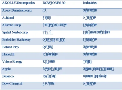
The source of the data used in this study is the Wharton Research Data Services. It includes annual data for the years 1995 until 2005 for 30 companies. There are nine variables included in the dataset and they are described in Table 2. Note, AKOLLY30 is an index that was created to mimic the DOW JONES 30. All the DJ30 industries are represented in the AKOLLY30 index with the same proportions. The main difference between the two indices is the companies included.
Table 2: Variables description
Variables Description
Dividend yield
(dp)
Dividend yield: I divided the annuals dividends by the year-end price of one share. Let d be the monthly dividend, I define dt as the annual
dividends in year t, i.e. the sum of all dividends issued throughout the year, hence the dividend yield is dt/pt
Log dividend
yield (ldp)
Logarithmic version of the dividend yield:ln(1+ dt/pt ).
E/P ratio(ep) It was calculated using the year-end earnings divided the year-end price per share
Log e/p
ratio(lep)
Logarithmic version of the e/p ratio: ln(1+ et/pt).
Book market
value( bm)
I use the year-end data. The book market-value is bt/pt, where pt is the
price per share at the end of year t and btis the book value of year t.
Log book
market value
( lbm)
Logarithmic version of the book market value: ln(1+ bt/pt)
Excess returns
(eret)
this paper. The formula for excess simple returns is (pt+dt)/pt-1
Log excess
returns ( leret)
Logarithmic version of the excess returns: ln((pt+dt)/pt-1).
year Year ranging from: 1995-2005
[image:17.612.68.490.85.291.2]age Number of years after IPO.
Table 3 lists the different companies in the various industries in the respective indices.
Table 3: Firms and Industries in AKOLLY30 and DJ30 Indices
AKOLLY30 companies DOWJONES 30 Industries
Avery Dennison corp. 3M Industrials
Ashland Alcoa Materials
Allstate Corp American Express Financials
Sprint Nextel corp. AT&T Telecommunication
Berkshire Hathaway Bank of America Financials
Eaton Corp. Boeing Industrials
HoneyIll Caterpillar Industrials
Valero Energy Chevron Energy
Apple Cisco Systems Information Technology
Pepsi co. Coca-cola Consumer Staples
[image:17.612.95.516.396.707.2]Halliburton co. Exxon Mobil Energy
General Dynamics General Electric Industrials
Dell Hewelet Packard Information Technology
McAfee IBM Information Technology
Intuit Intel Information Technology
Stryker corp. Johnson & Johnson Healthcare
Morgan Stanley JP Morgan Chase Financials
Tyson Foods Kraft Foods Consumer Staples
Target McDonald’s Consumer Discretionary
Boston Scientific Merck HealthCare
Citrix Systems Microsoft Information Technology
Bristol-Myers Pfizer Healthcare
Safeway Procter &Gamble Consumer Staples
Office Depot The Home Depot Consumer Discretionary
Capital one Travelers Financials
Raytheon United Technologies co. Industrials
Qwest Verizon Communications Telecommunication Serv.
Walgreen Wal-Mart Consumer Staples
Viacom Walt Disney Consumer Discretionary
3.2 General Diagnostics
Fixed effects will help us explore the relationship between the predictor and outcome variables within a company. Each company has its own characteristics, which can have an impact on returns. The most important assumption we make when using fixed effects within a company is that they may possibly impact the predictor or outcome variables, hence the need to control for it. This explains the assumption of correlation between error term and variables that may impact returns. In other words, the fixed effect model takes care of the time-invariants characteristics, in order for us to get the explanatory variables’ net effect. The other assumption of the fixed effect model is “that those time-invariant characteristics are unique to the individual and should not be correlated with other individual’s characteristics” (Oscar Reyna).
Unlike the fixed effect model, random effect model will assume that variations across companies are random and uncorrelated with the independent variables that are part of the model. The crucial distinction between fixed and random effects is whether the unobserved individual effect embodies elements that are correlated with the regressors in the model, not whether these effect are stochastic or not” (Green 2008). Do I have reason to believe that differences across companies have some influence on our dependent variables? If yes, then I should use the random effect model.
We use the Hausman’s test to decide which model to use. The null hypothesis is that the adequate model is the random effect model, and the alternative is the fixed effects model. The Hausman test or
Hausman specification test is a statistical test in econometrics named after Jerry A. Hausman. The
Pagan Lagrangier Multiplier test; whose null hypothesis is that variance across entities is zero (i.e. random effect is appropriate). The Breusch–Pagan LM test (named after Trevor Breusch and Adrian
Pagan) is used to test for heteroscedasticity in a linear regression model. It tests whether the estimated variance of the residuals from a regression are dependent on the values of the independent variables.
Suppose that we estimate the equation
(11)
We can then estimate , the residual. Ordinary least squares constrain these so that their mean is 0, so we can calculate the variance as the average squared values. A simpler method is to regress the squared residuals on the independent variables, which is the Breusch–Pagan test:
(12)
If an F-test confirms that the independent variables are jointly significant then I can reject the hypothesis of homoscedasticity, implying that there is heteroscedasticity.
The Breusch–Pagan test tests for conditional heteroscedasticity. It is a chi-squared test: the test statistic is
nχ2with kdegrees of freedom. If the Breusch–Pagan test shows that there is conditional heteroscedasticity,
it can be corrected by using the Hansen method, using robust standard errors, or re-thinking the regression equation. In the context of seemingly unrelated regression, Breusch-Pagan (1979) proposed a Lagrange Multiplier (LM) statistic, which is valid for fixed Nas T and is given by
LM=T (13)
(14)
And is the estimate of uit . LM is asymptotically distributed as chi-squared with N (N-1)/2degrees of
freedom under the null hypothesis of interest. However, this test is likely to exhibit substantial size distortions in cases where N is large and T is finite- a situation that is often encountered in empirical applications, primarily due to the fact that the Lm statistic is not correctly centered for finite T and the bias is likely to be worse with large N. With a test statistic of 0.06, I can reject the null and confirm our previous conclusion.
Next, we test for time fixed effect. We run a test to see if all time dummies are jointly equal to 0 (which is the null hypothesis) of an F-test, if they are then I do not need a time fixed effect model. With a test statistic of 0.0000, I reject the null, which indicates that a time fixed effect model is needed.
If there is a time fixed effect, it means that the variable “year” affect returns. It is safe to conclude that “year” might also affect dividends since dividends are also part of the return.
3.3 Empirical Analysis (Using Data Subset)
3.3.1 Dividends in Different Industrial Sectors
different industries. He concluded that, industry does not have any influence on managers’ point of view. This contradicts with the findings of Baker, Farrelly and Edelman (1985) that find out that there are concrete difference between utilities and manufacturing. Those results could be explained by greater competitive environment in utilities and regulations which has made the utilities industry riskier than before. Michel (1979) showed that there is a strong link between industry classification and dividend payout. Dhrymes and Kurz (1967), Mccabe (1979) and Michel (1979) have all shown evidence that a firm’s industry influence its dividend payout. The view of Higgins (1972) contradicts those of Michel. He finds no evidence that industry classification affects dividends. Rozeff (1982) solves the questions several ways, initially he examine the residual across all firms. The input of the data is done in order of industry. If there industry effects, they will manifest themselves by nonrandom variables, i.e. the residuals of the same sign and same industry group will be clustered together. He uses the DW11(Durbin-Watson) test;
the test statistic of 1.88 shows that there some randomness in the residuals which shows that there is no industry effects. Secondly, he selects 8 different industries with a minimum of thirty companies each. He ran regression on each of them, then he use Chow tests12to test if all the coefficients are equal. The
F-statistics ends up being too small and he ends up failing to reject the hypotheses that each industry has the
11
The Durbin–Watson statistic is a test statistic used to detect the presence of autocorrelation in the residuals from a regression analysis. It is named after James Durbin and Geoffrey Watson.If etis the residual associated with the observation at time t, then the test statistic is
Since dis approximately equal to 2(1-r), where ris the sample autocorrelation of the residuals,[1]d= 2 indicates no autocorrelation. The value of dalways lies between 0 and 4. If the Durbin–Watson statistic is substantially less than 2, there is evidence of positive serial correlation. As a rough rule of thumb, if Durbin–Watson is less than 1.0, there may be cause for alarm. Small values of dindicate successive error terms are, on average, close in value to one another, or positively correlated. If d> 2 successive error terms are, on average, much different in value to one another, i.e., negatively correlated. In regressions, this can imply an underestimation of the level of statistical significance.
12
same regression coefficient as the one in the pool sample model. Thirdly, he takes residuals from the regression of each individual industry and sees if they fall randomly around the regression line; if they do then there are no industry effects. Using a 5% confidence level, eight industries out of sixty four have residuals that are nonrandom. Those industries include Home Appliance, Fast Food Service, Securities Brokerage and Retail. Finally, he uses dummy variables for the eight industries mentioned previously and runs the regression. Six out the eight prove to be significant.
There are several issues with Rozeff’s approach. First, when he runs regression on industries dummies without other variables that might affect dividends among the explanatory variables, there is a model misspecification problem: There is some variability in dividends that cannot be captured by the dummy variable “industry” alone. Second, the industry classification by Rozeff is flawed in the sense that some of them can be grouped together, for instance the Home Appliance industry and the Toiletries/ cosmetics industries can be grouped together under the “consumer products” industries.
In this paper we solve those two shortcomings, by initially choosing four distinct industries. We make sure they do not have anything in common and are distinct in each of their main characteristics. The four industries selected are: Financials, Healthcare, Information Technology and Utilities.
We picked 19 companies from each of the four industries. Dummy variables are created from each industry: 1 for financial industry, 2 for healthcare, 3 for information technology and 4 for utilities. We include dummy variables for all the years based on the following grouping: 1 from 1995 to 1997, 2 from 1998 to 1999, 3 for 2000 to 2001, 4 for 2002 to 2003, and 5 for 2004 to 2005.
“dyear” and “ ldp”, in other words between year and dividend yield. In other words, does economic cycle (variable “dyear”) affect dividend yield (thus returns) on average. The same reasoning motivated the inclusion of the interaction variable “ind.ldp”. Does industry influence dividend yield? If yes, to what extent?
We start by running the Hausman’s test, in order to choose between fixed or random model. The test statistic of 0.000, suggests that we use a fixed effect model. We then checked for cross-sectional dependence and contemporaneous correlation: based on the Pesaran CD test. Pesaran (2004) has
proposed the following alternative to the Breusch-Pagan LM test:
CD= (15)
Where Tij= # (Ti Tj)(i.e. the number of common time series observations between units i and j),
(16)
and
= (17)
The test revealed a cross sectional dependence. In order to solve our cross sectional dependence problem, we will use the Driscoll and Kray standard errors’ method. Let consider the following linear regression
The dependent variable is a scalar, is a (K+1) x 1 vector of independent variables whose first
element is 1, and is (K+1) x 1 vector of unknown coefficients. is the cross-sectional unit
(“individuals”) and denotes time. We assume that the regressors
and the scalar disturbances are uncorrelated. We can thus consistently estimate by least squares (OLS)
regression:
= (18)
Driscoll and Kraay standard errors for the coefficient estimates are the square roots of the diagonal entries of the asymptotic (robust) covariance matrix.
(19)
where
(20)
where is the lag length up to which residuals may be autocorrelated. The (K+1) x (K+1) matrix
is defined as :
) ) (21)
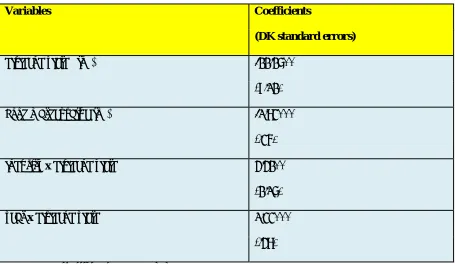
The advantage of running a regression with Driscoll and Kray standard errors is that in addition to fixing cross sectional dependence, we do not have to worry about heteroskedacity and autocorrelation. The output of the regression is displayed in Table 4.
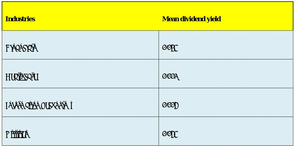
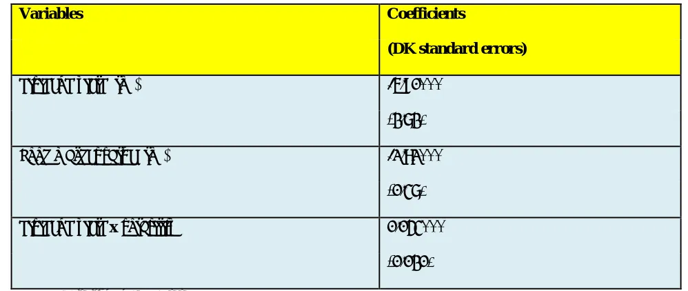
As expected, all the coefficients are significant, recall that ydp is the product of the year dummy and dividend yield, while idp is the product of industry dummy variable and dividend yield. The significance of the interaction variables’ coefficients implies that there is some interaction effect between the dividend yield and the two dummy variables. This suggests that the industry to which a firm belongs to affects its dividend thus its returns, which was our hypothesis earlier. The interaction effect between years and dividend yield could be hypothesized as older firms pay less dividend than younger firms. Why? This would make sense if paying dividend (thus high dividend yield) was in fact a signal mechanism; a way of attracting investors and getting the trust of the market. To answer those questions, we look at the mean dividend yield by industry. Table 5 displays the mean dividend yield by industry. There seems to be a vast difference between dividend yields paid by industries. How can that be explained? Why do financials and utilities have the highest dividends yields? We address those questions in two folds. Initially we hypothesize that dividends might be in fact a signaling mechanism; second we check if dividends can be considered a compensation for risk.
3.3.2 Dividends as a Signaling mechanism
Table 4: Dividends in different industries: Regression with Driscoll-Kraay standard errors of
excess returns on explanatory variables
Variables Coefficients
(DK standard errors)
dividend yield ( log) -22.27**
(9.12)
book market value(log) -1.83***
(.36)
industry xdividend yield 4.42**
(2.17)
year xdividend yield 1.33***
(.48)
Notes:***: significant at p<0.01 level.
**: significant at p<0.05 level.
The rationale being that a firm that has survived past recessions, competition, and change in its industry is more equipped to survive future challenges. Everything else equal, investors are willing to invest in that firm. It is fair to assume that everything else equal, investors will more likely invest in firms that have been around longer. For instance, most casual investors are more likely to invest in IBM than in a new start up in Silicon Valley. If we follow that rationale, we could use age of the company as a proxy to ability to survive in competitive market place. Let age be the number of years since the IPO13.
13According to Gregoriou (2006) an
initial public offering(IPO) referred to simply as an "offering" or "flotation," is when a company
[image:27.612.72.527.144.408.2]Table 5: Mean Dividend Yield by Industry
Industries Mean dividend yield
Financials 0.023
Healthcare 0.001
Information Technology 0.004
Utilities 0.043
Our assumption is that, in a capitalist market, firms that have been profitable survive through the years, while firms that have not been profitable either are bankrupt and disappeared or are taken over by more profitable companies. In summary I assume a sort of natural selection, where stronger (more profitable) firms survive, while the weaker(less profitable) firms are bankrupt or taken over. Miller and Modigliani (1961) showed that price per share is often an after effect of dividend rate. Powell (1999) affirms that due to information asymmetry between the corporate managers who has an information advantage and the investors, dividend might be a way to communicate the firm’s future profitability, or in a lesser extent its potential future profitability. On the other hand, investors will use the dividend announcement as a measure of the stock price. Are dividends perfect signals? Easterbrook (1994), affirms that increases in
dividends are “ambiguous”, unless the market can distinguish between growing firms and firms with lack of investments chances. To illustrate this point, Soter, Brigham, Evanson (1996) give the example of the parent company of Florida Power and Light Company. In 1994, the parent company, announced a 32%reduction in their quarterly dividend, the stock drop by 20%. It is only after, it was determined that the reduction in dividend was made not because of problem in cash flow, but because of strategic reasons to invest in the company’s growth. It is only after investors figured out this was the case that the stock recovered. Savov (2006) discuss the dividend-signaling hypothesis by analyzing the post-announcement performance of German companies. She specifically looks at characteristics such as earnings, level of earnings, assets growth, and capital expenditures. She also looks at the annual stock return and sees if signaling theory can be the cause of the negative correlation between the dividend decision and the stock price performance. Savov get results that go against the theory. She finds out that there is not “any evidence that dividend increases or convey information about the future operating performance”. Companies do not perform significantly better after the announcement of dividends’ paying. “Not only does earning not increase after a dividend increase, they do in fact decrease” Savov (2006). The limitations of the models used by Savov and Modigliani, is the fact that their proxy for successful companies is flawed: For instance using percentage change in dividend payments as a measure of success or profit has its limit as I showed it earlier. We consider 30 companies from the utilities industry. We create a variable “age” which is the age of the company at the time the dividend, earning
and other characteristics are released. Compared to the regression in the previous part, we use the same variables and interaction variables, but this time industry and year variables are not considered, the variable “age” is introduced. We regress excess returnson dividend yield, book market value, E/P ratio,
age and agex dividend yield. We control for industry by choosing firms from the same industry. The
that we should use a fixed effect model. The Pesaran cross-sectional dependence test suggests that there is a cross-sectional dependency. We will use Driscoll and Kray standard errors to fix it. The output is in Table6.
Table 6: Dividend as signaling mechanism: Regression with Driscoll-Kraay standard errors of
log-excess returns on explanatory variables
Variables
Coefficients
(DK standard errors)
Earning price ratio(log) -0.04
(0.12)
Dividend yield(log) -2.37
(2.99)
Book market value(log) -1.31***
(.32)
Age 0.024
(0.016)
Age x log dividend yield -0.015
(0.02)
Notes:***: significant at p<0.01 level.
market at the time. It is then justified that book-market value might be a better proxy of a firm’s health, since it encompasses verifiable assets and market’s sentiment at the exact time. Perhaps the use of book market value might be a good proxy for profit over.
In Table 6, after the utilities industry, financials was the second industry with the highest average dividend yield. It appears that risk might be a factor. Paying dividend might be a way of compensating for risk.
3.3.3 Dividends as Compensation for Risk
growth rate of dividends is related to the economy’s rate of output. This implies that dividend growth is equal to rate of interest. The dividend yield method of estimating risk states that: equity risk premium14is
proportional to dividend and inversely proportional to Treasury bill interest rate.
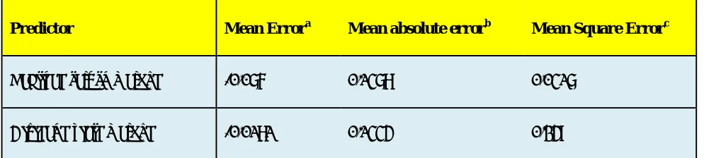
[image:32.612.70.567.297.409.2]This means that fluctuations in the equity risk premium can be measured by fluctuation in the dividend yield, since there is not much fluctuation in the Treasury bill’s interest rate. Comparisons between the two different methods are displayed in Table 7.
Table 7: Prediction Errors of Realized Return and Dividend Yield Methods, 1962-1982
Predictor Mean Errora Mean absolute errorb Mean Square Errorc
Realized return method -0.076 0.1378 0.0317
Dividend yield method -0.0181 0.1334 0.249
aDefined as arithmethic mean over 21 annual observations of (A-F
1) where A= actual risk premium and F1=forecasted risk premium.
bDefined as arithmetic mean of | A-F 1|.
cDefined as arithmetic mean of (A-F 1)2.
The forecasts of the realized return method have mean of 9.94%, while the mean realization was 2.34%. On the other hand the dividend yield method had a mean 4.15% which is very close to 2.34%. The average error for the realized return method is 13.8% versus 13.3% for the dividend yield methods. Our hypothesis, that dividend might be a compensation for risk is thus justified. Using the mean square error criterion, the dividend yield method’s MSE is .0249 compared to the .0317 of the realized risk return
14
methods. This has shown us the positive relationship between the dividend yield and the equity risk premium. This might explain why the utilities and the financial industries have the highest dividends. We hypothesize that dividend yield is in fact a compensation to the investor for taking risk. We will study and verify this hypothesis by observing the volatility of different companies in various sectors.
We observe 19 firms in 5 different industries. Here we will define volatility or risk by variance in price per share; we then run a regression of excess returns on E/P ratio, dividend yield, book market value,
volatilityand volatilityxdividend yield. The Hausman’s test suggest that I use a fixed effect model( test
statistic of 0.000).The Pesaran CD test reveal a cross sectional dependence( test statistic of 0.000).To fix it we will use the Driscoll and Kay variances. The output is in Table 8, volatility’s coefficient became insignificant and was dropped, however the interaction variable’s coefficient riskyield which is the product between dividend yield and volatility is significant which tell us that there is some interaction effect between the dividend yield and the volatility and it affects excess returns.
Table 8: Dividend as compensation for risk: Regression with Driscoll-Kraay standard errors of
excess returns on explanatory variables
Variables Coefficients
(DK standard errors)
dividend yield (log) -5.90***
(2.72)
book market value (log) -1.81***
(0.37)
dividend yield xvolatility 0.043***
(0.020)
Notes:***: significant at p<0.01 level.
3.3.4 Excess Return Model
Earlier we have investigated variables that might influence dividend yield. We found out that volatility, years in industry, year’s economy and type of industry all influence dividend yield. Can we extend that conclusion to excess returns? It would be a legitimate extension since we know that dividend is included into returns. We include all the variables I have studies earlier that affect dividend yield into this last regression. We are expecting better predictability. The Hausman’s test suggest a fixed effect model and the Pesaran CD test reveals a cross sectional dependence. We use the DK variances methods; our output is in Table 9.
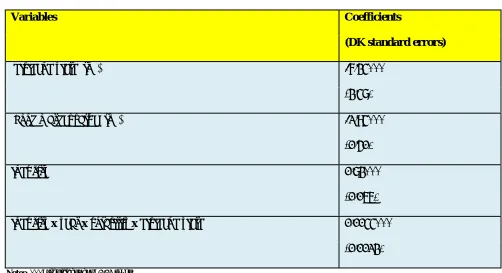
Of all the variables studied, the significant ones are log dividend yield, log book market value, industry
and industry x year x volatility x dividend yield. The dividend yield (log), which was expected since
[image:34.612.63.562.145.356.2]Table 9: Excess return model: Regression with Driscoll-Kraay standard errors of excess returns
explanatory variables
Variables Coefficients
(DK standard errors)
dividend yield (log) -6.23***
(2.37)
book market value (log) -1.83***
(0.40)
industry 0.72***
(0.055)
industry xyear xvolatility xdividend yield 0.0033***
(0.0012)
Notes:***: significant at p<0.01 level.
[image:35.612.66.568.138.411.2]competitor. Finally, the interaction variable between industry, year, volatility and dividend yield is significant. First it tells us that those variables influence each other. Second, the variable that deserves attention is year, since it is the only that has not been studied so far. Depending on the year, stocks prices might be rallying or retracting. year encompasses more parameters than can affect the markets and consumers, thus returns. For instance depending on the year, we might have the Federal Reserve lower interest rate. We might be in election’s year or in a recession or in a war, all of which can affect a firm’s performance in particular and the economy as a whole. All the variables that we have hypothesized as being determinants of returns have been proven to be significant.
Conclusion
insignificant in predicting returns; book market value is a much better predictor. If investors have paid attention to the book market value as our study suggested, they would have noticed accounting irregularities and avoid the stock. In our study, we showed that dividends were compensations for risk. A good illustration of that fact is the collapse of BP’s stock price. BP being in a risky industry-the energy industry- has a history of paying dividend. As a result, the stock price was high. However, the oil spill in the Gulf of Mexico on April 22nd2010 sent a shockwave through the market, lowering BP’s stock price. It
References
Baker, Kent, Gail Farelly, and Richard Edelman, “A Survey of Management Views on Dividend Policy”,
Financial Management, 1985, Vol.14, No. 3, pp 78-84.
Breusch, T.S.; Pagan, A.R. ,"Simple test for heteroscedasticity and random coefficient variation".
Econometrica(The Econometric Society), 1979, 47 (5): 1287–1294.
Campbell, John Y. and Robert Shiller, “The Dividend-Price Ratio and Expectations of Future Dividends and Discount Factors”, Review of Financial Studies, 1988a, Vol1, No 3 pp 195-228.
Dhrymes, PJ and, Mordecai Kurz, “Investment, Dividend, and external finance behavior of firms:, NBER
chapter, 1967, pp 427- 486.
Driscoll, J.C. and A.C. Kraay, “Consistent Covariance Matrix Estimation with Spatially Dependent Panel Data”. Review of Economics and Statistics, 1998, Vol. 80, pp549-560.
Fama, Eugene and Kenneth French, “Dividends Yields and Expected Stock Returns”, Journal of
Financial Economics, 1988, 22, pp.3-25.
Gordon, M.J., the Investment, Financing, and Valuation of the Corporation, Irwin, Homewood, Ill. 1962.
Hausman, J.A. “Specification Tests in Econometrics”, Econometrica, 1978, 46 (6), 1251-1271,
Higgins, Robert, “Dividend Policy and Increasing Discount Rates: A Clarification”, Journal of Financial
and Quantitative Analysis, 1972, Vol.7, No.3 pp 1757-1762.
Ibbotson, R.G., and R.A. Sinquefield, “Stocks, Bonds, Bills and Inflation: The Past and The Future”,
Financial Analysts Research Foundation, 1982.
Lamont, Owen, “Earnings and Expected Returns”, Journal of Finance, Vol. 53, No 5 (Oct.1998), pp.1563-1587.
Michel, Allen, “Industry Influence on Dividend Policy”, Financial Management, 1979, Vol.8, No. 3, pp 22-26.
Miller, M., and F. Modigliani, “Dividend Policy Under Asymmetric Information,” Journal of Finance,40, 1031-1051.
Pesaran, “General diagnostic tests for cross section dependence in panels", Cambridge Working Papers in
Economics,(2004), No. 0435.
Peterson, Pamela, “Analysis of Financial Statements”,Wiley, (1999), p. 92.
Powell Gary, “How Corporate Managers View Dividend Policy”, Quarterly Journal of Business and
Economics, 1999, Vol.38.
Savov, Sava, “Dividend Changes, Signaling, and Stock Price Performance”, Mannheim Finance Working
Paper, 2006, No 3.
Shiller, Robert, “Stock Prices and Social Dynamics”, Brookings Papers on Economic Activity, 1984:2, 457-498.
Silvey, S. D., “The Lagrangian Multiplier Test”, Annals of Mathematical Statistics30, 1959, 389-407.
Soter, Brigham, Evanson,” The Dividend cut heard around the World”, Journal of Applied Corporate