Estimation of Dynamic Discrete Games Using the Nested Pseudo Likelihood Algorithm: Code and Application

(1)

Munich Personal RePEc Archive

Estimation of Dynamic Discrete Games

Using the Nested Pseudo Likelihood

Algorithm: Code and Application

Aguirregabiria, Victor

University of Toronto, Department of Economics

15 September 2009

Online at

https://mpra.ub.uni-muenchen.de/17329/

(2)

Estimation of Dynamic Discrete Games Using the

Nested Pseudo Likelihood Algorithm: Code and Application

Victor Aguirregabiria

∗∗

University of Toronto

August 20, 2009

Abstract

This document describes program code for the solution and estimation of dynamic discrete games of incomplete information using the Nested Pseudo Likelihood (NPL) method in Aguir-regabiria and Mira (2007). The code is illustrated using a dynamic game of store location by retail chains, and actual data from McDonalds and Burger King.

TABLE OF CONTENTS

1. Introduction

2. Empirical Application

2.1. Model

2.2 Data

2.3. NPL Method

3. Main Program (npl_dyngame.prg)

Part 1: Speciﬁcation of Some Constants.

Part 2: Reading data. Construction of vectors of observed states and decisions

Part 3: Procedures

Part 4: Initial Estimates of Conditional Choice Probabilities Part 5: NPL Estimation

4. Procedures

4.1. freqprob

4.2. miprobit

4.3. npl_bkmd

5. Output and Empirical Results

Appendix: Gauss code

(3)

1 Introduction

This document describes program code for the solution and estimation of dynamic discrete games

of incomplete information using the Nested Pseudo Likelihood (NPL) method in Aguirregabiria

and Mira (2007). The code is written in GAUSS programming language and it is included in

an Appendix and available online at http://individual.utoronto.ca/vaguirre/. Given that

the code uses low-level commands in GAUSS, it should be straightforward to translate it to other

matrix languages such as Matlab, Fortran 90, R, or C+. I illustrate the use of this software using a

dynamic game of store location by retail chains and actual data for McDonalds and Burger King.

The example is intentionally simple and it tries to provide a helpful starting point for the user of

this code. The list of programs (.prg) and procedures (.src) is the following:

Program / Procedure Description

npl_dyngame.prg Main program for the NPL estimation of a dynamic game of store location

npl_bkmd.src Given an initial vector of choice probabilities (CCPs), it computes an NPL

ﬁxed point estimator.

miprobit.src Given a vector of choice probabilities (CCPs), it returns the pseudo ML estimator of a probit model.

freqprob.src Calculates a frequency estimator of Conditional Choice Probabilities (CCPs)

The main program isnpl_dyngame.prg. It includes all the procedures that it calls, such that the

user does not have to create any GAUSS library with the procedures called by the main program.1

The rest of this document is organized as follows. Section 2 presents the model, data, and

the estimation method in the empirical application that we use to illustrate the algorithm and

code. Section 3 describes the diﬀerent parts of the main program. Section 4 goes through the procedures or subroutines called by the main program. Section 5 describes the estimation output

and comments the estimates in the empirical application. The code is included in an Appendix.

1_{Alternatively, the user might prefer to remove from the main program all the procedures and place them in a}

(4)

2 Empirical Application

2.1 Model

Time is discrete an indexed by t _∈ {1,2, ..., T}, where T is the time horizon. There are two

players in the game, and we use the indexesi_∈{1,2} and j_∈{1,2} to represent a player and his

opponent, respectively. Every period, each player makes a binary choice. Within a given period

players’ actions are taken simultaneously. LetYit∈{0,1}represent the choice of playeriat periodt.

Each player makes this decision to maximize its expected and discounted payoﬀEt(PT_s=0−tβ

s

iΠi,t+s), whereβ_i _∈(0,1)is playeri’s discount factor andΠit is his payoffat period t. Here we concentrate in Markovian decision models with infinite horizon,T =_∞. The payofffunction has the following structure:

Πit =zit(Yit, Yjt) θi−Yit εit (1)

z_it₍₀_,₀₎_, z_it₍₀_,₁₎_, z_it₍₁_,₀₎_{, and} z_it₍₁_,₁₎ _{are row vectors of known functions of state variables.} _θ_i

is a column vector of structural parameters, and θ ≡ (θ1,θ2) is the vector with both players’

parameters. Structural parameters and the vectors z_it₍_Y_it_{, Y}_jt₎ _{are common knowledge to the two}

players, up to the action of the other player. The variable εit is private information of ﬁrm i at

periodt. A player has uncertainty on the current value of his opponent’s ε, and on future values

of both his own and his opponent’sε0s. The vectors z_it₍_Y_it_{, Y}_jt₎ _{have the following structure:}

z_it₍_Y_it_{, Y}_jt_{) =}_z₍W_i_{, X}_it_{, X}_jt_{, Y}_it_{, Y}_jt₎ ₍₂₎

z() is a known vector-valued function. W_i _{is a vector of time-invariant exogenous characteristics}

of playeri. AndXitis an endogenous ’stock’ variable for playerithat evolves over time according

to the transition ruleXit+1 =Xit+Yit. The set of possible values for these stock variables is{0,1,

2, ..., K} where K >1 is a natural number that represents the maximum level of the stock. The

variables ε1t and ε2t are independent of (W1,W2), independent of each other, and independently

and identically distributed over time. Their distribution functions, G1 and G2, are absolutely

continuous and strictly increasing with respect to the Lebesgue measure onR.

The model can easily accommodate depreciation (e.g.,Xit+1 = (1−δ)Xit+Yit, with0< δ <1)

(5)

illustrate the algorithm and code, the two retail chains never closed a store during the sample

period. Therefore, we have preferred to present here the simple case without depreciation or

disinvestment because that is the case in the empirical application.

EXAMPLE (Capacity Investment in an Oligopoly Industry). Consider a dynamic game of capacity

investment between twoﬁrms competing in an oligopoly industry of an homogeneous product.2 The

demand function is Qt =St(b0−b1Pt), where b0 and b1 are parameters, Qt represents aggregate

output, St is the exogenous market size, andPt is the product price. There are 2 ﬁrms operating

in the industry. Every period t, theseﬁrms compete in quantities a la Cournot (static game), and

choose whether to invest to increase their capacity (dynamic game). Production costs are linear

in the quantity produced, i.e.,Cit=M Cit qit, whereM Cit is the marginal cost, and qit represents

output. Marginal cost declines with installed capacity, i.e., M Cit=ci−d(Xit+Yit), where ci >0

andd >0are parameters,Xitis the installed capacity at the beginning of periodt, andYit ∈{0,1}

represents capacity investment, that is a binary choice. It is simple to show that the Cournot

equilibrium variable proﬁt ofﬁrmiis:

V Pit = St b1

µ

b0+M Cjt−M Cit

3

¶2

= θV P0i St 1{Xit+Yit>0}+θV P1i St(Xit+Yit−Xjt−Yjt) +θV P2i St(Xit+Yit−Xjt−Yjt)2 (3)

where 1{.} is the indicator function, and θV P0i >0, θV P1i , and θV P2i are structural parameters that

are known functions of the ’deep’ parameters b0,b1,ci,cj, andd. More speciﬁcally, it is simple to

verify thatθV P0i ≡(b0+cj−ci)2,θV P1i ≡2d(b0+cj−ci), andθV P2i ≡d2. Given a value of the vector

of parameters(θV P0i ,θV P1i ,θV P2i :i= 1,2), we can (over-)identify the ’deep’ structural parametersd,

b0, and(cj−ci). Here we concentrate on the identiﬁcation and estimation of the parameters(θV P0i ,

θV P1i ,θV P2i :i= 1,2)together with the parameters inﬁxed costs.3 The set of possible capacity levels

2_{See Besanko and Doraszelski (2004), or Ryan (2009) for related dynamic games of}

ﬁrm capacity.

3

We may consider a more flexible model of competition between McDonalds and Burger King. Suppose that thesefirms have differentiated products. The demand function form firm iis qi =Ai−b(Pi−Pj), whereAi and

bare structural demand parameters. The specification of the marginal cost function is the same as above. Firms compete in prices a la Nash-Bertrand. It is straightforward to show that variable profit offirmiin the Nash-Bertrand equilibrium is:

V Pi = S

b

2Ai+Aj+b(MCi−MCj) 3

2

(6)

is{0,1,2,...,K}whereK₋1>1is a natural number that represents the maximum feasible level

of capacity. Aﬁrm’s capacity evolves over time according to the transition rule Xit+1 =Xit+Yit.

The ﬁrm’s total proﬁt function is:

Πit=V Pit−θF C0i 1{Yit+Xit>0}−θF C1i (Yit+Xit)−θF C2i (Yit+Xit)2−Yit εit (4)

where θF C0i , θF C1i and θF C2i are parameters in the ﬁxed cost function of ﬁrm i. The variable εit is

a private information shock in the ﬁrm’s investment cost, and it is normally distributed. In this

example, the vector of structural parameters forﬁrmi is:

θi ≡(θV P0i , θV P1i , θV P2i , θF C0i ,θF C1i , θF C2i )0 (5)

and the vectorZ_it₍_Y_it_{, Y}_jt₎ _is:

Z_it₍_Y_it_{, Y}_jt₎ _≡ ©_S_t₁_{_X_it₊_Y_it _>₀_}_,_S_t₍_X_it₊_Y_it₋_X_jt₋_Y_jt₎_,_S_t₍_X_it₊_Y_it₋_X_jt₋_Y_jt₎2

(₋1{Xit+Yit>0}, −(Xit+Yit), −(Xit+Yit)2

ª

(6)

In our empirical application, we consider the industry of fast-food burger restaurants in UK.

The two companies are McDonalds and Burger King who compete in the number of stores. A local

market is a district. Xit represents the number of installed stores, and Yit is the decision to open

a new store. During the sample period (1991-1996), these ﬁrms did not close any existing store.

That is the reason why there is not an exit decision in the model. The model assumes that the

decision to open a new store is completely irreversible.

Players’ strategies are the result of a Markov Perfect Equilibrium (MPE). In a MPE, players’

strategies depend only on payoff relevant state variables. In this model, the payoff-relevant infor-mation of firm i at period t is (St, X1t, X2t, εit). We use Xt to represent the vector of common

knowledge state variables: X_t _≡ ₍_S_t_{, X}₁_t_, _X₂_t_{). Let} _X _{be set with all the possible values of} X_t_.

Let σ _≡{σi(Xt, εit) : i= 1,2} be a set of strategy functions, one for each player. σ is a MPE if,

for every player i, the strategy σi maximizes the expected value of ﬁrm i at every state (Xt, εit)

and taking as given the opponent’s strategy. It is convenient to represent players’ strategies and

MPE in terms of players’Conditional Choice Probabilities (CCPs). Let Pi(Xt)represents ﬁrm i0s

(7)

probability of increasing its capacity (i.e., of Yit = 1) given that the state is Xt. This probability

is deﬁned as the integral of the strategy functionσi(Xt, εit) over the distribution ofεit.

Pi(Xt)≡

Z

1{σi(Xt, εit) = 1} dG1(εit) (7)

where 1{.} is the indicator function. We can represent a MPE as a pair of probability functions

P_≡_{_P_i₍X_t_{) :}_i_{= 1}_,_2; X_t_∈_{X }} _{such that the strategy} _P_i _{maximizes the expected value of} _ﬁ_rm_i

at every stateX_t_{taking as given the opponent’s strategy} _P_j_.

The equilibrium mapping in the space of CCPs is the key component of this class of dynamic

games. It summarizes all the relevant structure in the model. The form of this equilibrium mapping

depends on the payoff function, the transition rule of the state variables, and the distribution of the private information shocks εit. As shown above, in our model the one-period profit of firm i

can be written asΠit=Zit(Yit, Yjt)θi−Yit εit. Therefore, the one-periodexpected proﬁt of ﬁrmi

is:

ΠP

it(Yit) = (1−Pj(Xt)) Zit(Yit,0)θi+Pj(Xt) Zit(Yit,1)θi−Yitεit

= zP

it(Yit) θi−Yitεit

(8)

where zP

it(Yit) ≡(St, St(Xit+Yit),(1−Pj(Xt))St(Xjt+ 0) +Pj(Xt))St(Xjt + 1),−Yit,−YitXit). For the sake of illustration, let us consider ﬁrst the equilibrium mapping for the case when ﬁrms

are myopic, i.e., β1=β2= 0). The best response function in the space of a player’s action is:

{Yit= 1}⇔©zPit(1)θi−εit≥zPit(0) θiª (9)

And in the space of CCPs, ﬁrmi’s best response is:

Pr (Yit= 1|Xt) =Gi

¡£

zP_it₍₁₎₋zP_it₍₀₎¤_θ_i¢ ₍₁₀₎

A MPE in this static/myopic game (i.e., a Bayesian Nash Equilibrium) is a pair of probability

functions that solves the system of equations:

P1(Xt) = G1

¡£

zP

1t(1)−z

P

1t(0)

¤

θ1

¢

P2(Xt) = G2

¡£

zP₂

t(1)−z

P

2t(0)

¤

θ2

¢ (11)

for every value of X_{t. Given our assumptions on the distributions} _G_{i, Brower’s Theorem implies}

(8)

or static game, there is a separate system of equations for every value of X_t_{. We could say that}

for each value of X_t _{we have a separate equilibrium. As shown below, this is not the case for a}

dynamic game. In a MPE of a dynamic game, the whole best response probability function of

player idepends on the whole probability function of playerj at every possible value of X_t_.

Now, we describe a MPE in a dynamic game where players are forward-looking, i.e., β_i >

0. Following Aguirregabiria and Mira (2007), a MPE can be described as a vector of CCPs,

P_≡_{_P_i₍X_t_{) :}_i_{= 1}_,_2; X_t_∈_{X }}_{, such that for every} _ﬁ_rm _i_{and every state}X_t_∈_X _{we have that:}

Pi(Xt) = Gi

¡£ e

zP

it(1)−ez

P

it(0)

¤

θi−

£ e

eP

it(1)−ee

P

it(0)

¤¢

(12)

whereezP

it(Yit)is the expected and discounted sum of current and futurezvectors{zit+s(Yit+s, Yjt+s) : s= 0,1,2, ...}which may occur along all possible histories originating from the choice ofYitin state

X_{t, if every player behaves according to their CCPs in}P_{. More formally,}

e

zP

it(Yit)≡ zPit(Yit) + E

Ã_∞

X

s=1

βs zP

it+s(Yit+s) |Xt, Yit

!

(13)

Similarly, _eeP

it(Yit) is the expected and discounted sum of realizations of{εit+sYit+s :s= 0,1,2, ...} originating from the choice of Yit in state Xt, when players behave according to their CCPs in P:

e

eP

it(Yit) ≡ E

Ã_∞

X

s=1

βs εit+sYit+s |Xt, Yit

!

(14)

Now, we describe in detail the exact computation of the values_ezP

it(0),ez

P

it(1),ee

P

it(0), andee

P

it(1),

for every possible value ofX_t_{in the space of}_X_{. Let}_fP

i (Xt+1|Yit,Xt)be the transition probability of {X_t_} _{from the point of view of player} _i_{who knows his own current action} _Y_it _{but ignores the}

current action of his competitor and only knows that it is a random draw from the probability

distributionPj(Xt). By deﬁnition,

f_iP(X_t+1|Yit,Xt)≡1{Xit+1=Xit+Yit} Pj(Xt)1{Xjt+1=Xjt+1}(1−Pj(Xt))1{Xjt+1=Xjt} (15)

Deﬁne also the value vector WP

Z_i(Xt) ≡ (1−Pi(Xt))ez P

it(0) +Pi(Xt)ezPit(1), and the scalar value WP

ei(Xt)≡(1−Pi(Xt))eePit(0) +Pi(Xt)eePit(1). It is straightforward to see that, by deﬁnition:

ezP

it(Yit)≡ zPit(Yit) + β

X

X_t₊₁_∈_X

fP

(9)

and

e

eP

it(Yit) ≡ β

X

X_t₊₁_∈_X

fP

i (Xt+1|Yit,Xt) W_eiP(Xt+1) ₍₁₇₎

The matrix of valuesW_ZP

i ≡{W

P

Z_i(X) :X∈X }and the vector of valuesW P e_i ≡{W

P

ei(X) :X∈X } are obtained by solving systems of linear equations with dimension |X |. The solution to these

systems of equations has the following closed-form analytical expression:

W_ZP

i =

¡

I₋_β FP_X¢−1£₍₁₋P_i₎_∗ZP

i (0) +Pi∗ZPi (1)

¤ (18) and WP ei = ¡

I₋_β FP_X¢−1eP

i (19)

P_i _{is a} _{|X | ×}₁ _{vector with the stacked CCPs of player} _i _{for every possible value of} X_t_. ZP

i (0)

and ZP

i (1) are matrices with |X | rows and the same number of columns as z

P

it(Y) such that a

row of ZP

i (Y) is equal to the vector z

P

it(Y) associated with a given value of Xt. ∗ represents the Hadamard or element-by-element product. I _{represents the identity matrix with dimension} _{|X |}_.

FP

X is the transition matrix of {Xt} induced by the vector of CCPs P such that the elements

of this matrix are (1₋Pi(Xt))fiP(Xt+1|0,Xt) + Pi(Xt))fiP(Xt+1|1,Xt), or what is equivalent,

Q2

i=1Pi(Xt)

1{Xit+1=Xit+1}₍₁₋_P

i(Xt))1{Xit+1=Xit}. Finally, ePi is a vector that contains the ex-pected valuesE(εitYit|Xt, Yitis optimal)for every value ofXt. These conditional expectations only

depend on the probability distribution of εit and on the choice probability Pi(Xt). For the logit

and probit models we have the following closed expressions. Whenεit is extreme value distributed

(logit):

E(εitYit|Xt, Yit optimal) =Euler−(1−Pi(Xt)) ln (1−Pi(Xt))−Pi(Xt) ln (Pi(Xt)) (20)

whereEuler represents Euler’s constant. And whenεithas a standard normal distribution (probit):

E(εitYit|Xt, Yit optimal) =φ

¡

Φ−1(Pi(Xt))

¢

(21)

whereφ(.) andΦ−1

(.) are the PDF and the inverse-CDF of the standard normal.

Equation (12) represents a MPE as a ﬁxed point of a mapping in the space of CCPs. Given

our assumptions, Brower’s Theorem guarantees the existence of a MPE. In general, there may be

(10)

2.2 Data

To illustrate the algorithm and code, we estimate a dynamic game of store location by McDonalds

(MD) and Burger King (BK) using data for United Kingdom during the period 1991-1995. The

dataset comes from the paper Toivanen and Waterson (2005).4 It is a panel of 422local markets

(districts) andﬁve years with information on the stock of stores and the ﬂow of new stores of MD

and BK in each local market, as well as local market characteristics such as population, density, age

distribution, average rent, income per capita, local retail taxes, and distance to the headquarters

of the ﬁrm in UK.

We index ﬁrms by i∈ {BK, M D}, local markets by m, and years by t. The speciﬁcation of

the model is the one in the Example on Capacity Investment in an Oligopoly Industry in section

2.1 above. Ximt represents the number of installed stores ofﬁrm iin marketm at the beginning of

the year. The maximum value ofXimt in the sample is13, and we consider that the set of possible

values ofXimt is{0,1, ...,15}. Therefore, the state spaceX is {0,1, ...,15} × {0,1, ...,15} that has

256 grid points. Yimt is the binary indicator of the event "ﬁrm i opens a new store in market m

at yeart". For the code that we provide here, we consider that market characteristics are constant

over time, and use market-speciﬁc mean values of these variables. However, it is straightforward

to extend the code to accommodate exogenous state variables that evolve over time according to

ﬁrst order Markov processes. The measure of market size Sm is total population in the district. For some speciﬁcations, we allow the cost of investment to depend on market characteristics such

as average rent, retail taxes, population density, or average income.

2.3 NPL Estimation

For an arbitrary vector of players’ CCPs, P_≡_{_P_i₍X_{) :} _i _{= 1}_,_2; X _∈ _{X }}_{, de}_ﬁ_{ne the pseudo}

log-likelihood function:

Q(θ,P_{) =}

M P m=1 2 P i=1 T P t=1

Yimt lnGi

¡£ e

zP

imt(1)−ez

P

imt(0)

¤

θi−

£ e

eP

imt(1)−ee

P

imt(0)

¤¢

+ (1₋Yimt) ln

¡ 1₋Gi

¡£ e

zP

imt(1)−ez

P

imt(0)

¤

θi−

£ e

eP

imt(1)−ee

P

imt(0)

¤¢¢

(22)

(11)

In this likelihood function, choice probabilities are best responses to an arbitraryP_{. The arbitrary}

probabilities in P _{may be interpreted as players’ beliefs about other players’ expected behavior.}

These beliefsP _{are parameters to estimate together with} _θ_{. When} _G_i _{is the logistic function (or}

the CDF of the standard normal), the functionQ(θ,P₎ _{is the likelihood of a Logit (Probit) model}

where the parameter associated with the explanatory variableeeP

imt(1)−ee

P

imt(0)is restricted to be

−1. For every possible value of P_{, the likelihood} _Q₍_θ_,P₎ _{is globally concave in} _θ_{. This property}

simpliﬁes signiﬁcantly the implementation of the NPL algorithm.

LetP0 _{be the true vector of CCPs in the population under study, and let}Pˆ0_{be a nonparametric}

consistent estimator of P0_{. For instance, a frequency estimator of} P0 _is:

ˆ

P_i0(X_{) =}

PM m=1

PT

t=1Yimt 1{Xmt=X}

PM m=1

PT

t=11{Xmt=X}

(23)

The two-step estimator is deﬁned as the value ofθ that maximizes the pseudo likelihoodQ(θ,Pˆ0₎_.

The estimator is consistent and asymptotically normal. Its main computational cost is in the

calculation of the present values ezP_imtˆ0 _and _e_eP_imtˆ0 _{following the procedure described in section 2.1.}

However, for the example we consider here the dimension of the state space X is small and the

computation of these present values is quite simple. The main limitations of the two-step estimator

are its asymptotic ineﬃciency, its large ﬁnite sample bias, and its problems to accommodate unob-served variables for the econometrician which are common knowledge to players, such as unobunob-served

market characteristics.

If the equilibrium that generates the data is Lyapunov stable,5 then a recursive version of the

two-step estimator, i.e., a K-step estimator, has better asymptotic and ﬁnite sample properties

than the two-step estimator (see Aguirregabiria and Mira, 2007 and 2009, and Kasahara and

Shimotsu, 2008). Given an initial nonparametric estimatorPˆ0_{, the sequence of K-step estimators}

{ˆθK,PˆK _:_K _≥₁_} _{is de}_ﬁ_{ned as:}

ˆ

θK = arg max Q(θ,PˆK−1₎ ₍₂₄₎

5_Let

P=Ψ(θ,P)be theﬁxed point problem that deﬁnes an equilibrium for a given vector of structural parameters

θ. In our model, the equilibrium mappingΨ(θ,P)is Gi([zPit(1)−zitP(0)]θi−[ePit(1)−ePit(0)])for every playeriand

(12)

where the probabilities inPˆK _{are updated using the recursive formula}

ˆ

P_iK(X_t_{) =} _G_i

³h ezPˆK−1

it (1)−ez

ˆ PK−1

it (0)

i

ˆ

θK₋heePˆK−1

it (1)−ee

ˆ PK−1

it (0)

i´

(25)

This recursive procedure is called theNested Pseudo Likelihood (NPL) algorithm. The limit K-step

estimator, asK goes to inﬁnity, is anNPL ﬁxed point associated with the initial estimatorPˆ0_{. In}

general, an NPL ﬁxed point (ˆθNP L−F P,PˆNP L−F P) is deﬁned by two conditions: (1)θˆNP L−F P =

arg max Q(θ,Pˆ_{NP L}

−F P); and (2) PˆNP L−F P is an equilibrium of the model given ˆθNP L−F P. The model may have multiple NPL ﬁxed points. If the equilibrium that generates the data is

Lyapunov stable, then aNPLﬁxed point that is obtained by initializing the NPL algorithm with a

consistent initial estimatorPˆ0 _{is consistent, asymptotically normal, and it has smaller asymptotic}

variance and ﬁnite sample bias than the two-step estimator. If a NPL ﬁxed point is obtained by

initializing the NPL algorithm with an inconsistent initial Pˆ0_{, then the} _NPL ﬁxed point is not

necessarily consistent. In that context, theNPL estimator is deﬁned as the NPL ﬁxed point with

the largest value of the pseudo likelihood function. TheNPL estimator is consistent, asymptotically

normal, and it has smaller asymptotic variance andﬁnite sample bias than the two-step estimator

(Aguirregabiria and Mira, 2007).

The NPL method has been used in diﬀerent applications of empirical games or single-agent dynamic decision models, such as models of entry in oligopoly markets (Aguirregabiria, Mira,

and Roman, 2007, and Suzuki, 2008), plant turnover and productivity (Collard-Wexler, 2008,

and Tomlin, 2009), supermarket pricing strategies (Ellickson and Misra, 2008, and Kano, 2006),

dynamic games of competition between airline networks (Aguirregabiria and Ho, 2009), competition

between real estate agents (Han and Hong, 2008), adoption of new technologies (Lenzo, 2007), land

use and deforestation (De Pinto and Nelson, 2007 and 2009), quality competition between nursing

homes (Lin, 2008),ﬁrm investment (Sanchez-Mangas, 2002), entry and competition in the religion

industry (Walrath, 2008), demand of durable goods (Lorincz, 2005), or dynamic labor demand

(13)

3 Main Program (

npl_dyngame.prg

)

The ﬁle npl_dyngame.prg contains the main program where all the primitives are speciﬁed and

the diﬀerent procedures are called. This program is divided intoﬁve parts.

PART 1: Speciﬁcation of Some Constants.

The user should specify the values of the following constants and parameters.

Program Constant Description

filedat Name and address of the datafile. nvar Number of variables in the datafile. nobs Number of observations in the datafile. nmarket Number of markets in the dataset.

nyear Number of years in the dataset.

maxstore Maximum number of stores (i.e., max, value ofXit) namesb1 Vector with names of parameters that vary acrossﬁrms namesb2 Vector with names of parameters that do not vary acrossﬁrms nplayer Number of players

maxiter Maximum number of iterations for the NPL algorithm dfact Discount factor parameter,β

Given this information, the program generates the matrix vstate with all the possible values of

the vector of state variables X_t_{. Each row of} _vstate_{represents one value of} ₍_X₁_mt_{, X}₂_mt₎_.

PART 2: Reading Data and Construction of Vectors with observations of state and

decision variables

The vectors x_bk and x_md contain the observations of the state variables X1mt and X2mt. The

vectors a_bk anda_md contain the observations of the decision variables Y1mt and Y2mt.

PART 3: Procedures

This part of the program contains the diﬀerent procedures called by the main program: freqprob, procedure for the initial estimates of CCPs; miprobit, procedure for the maximum likelihood

estimation of a Probit model with constrains on parameters; andnpl_bkmd, procedure for the NPL

algorithm.

(14)

It calls the procedure freqprob for the frequency estimation of CCPs. In the version of the

program that we provide here by default, initial CCPs are estimated separately market by market.

Alternatively, the user could include time invariant market characteristics (i.e., population, average

income, density, etc) as explanatory variables and call the procedure freqprob only once but

including all the markets. The user could also prefer to use a Kernel estimator instead of the

frequency estimator.

By running this part of the program, we get a vector of estimated initial CCPs calledprob_freq.

Alternatively, if we want to search for multiple NPL ﬁxed points, we can replace this estimated

vector by an arbitrary value of prob_freq. For instance, initialized the NPL algorithm with a

vec-tor of constant probabilities, e.g.,prob_freq = (1/2)*ones(nmarket*nstate,nplayer);, or with

random draws from a uniform distribution, e.g.,prob_freq = rndu(nmarket*nstate,nplayer);.

PART 5: NPL Estimation.

This part of the program calls the procedure for NPL estimation,npl_bkmd, that generatesmaxiter

iterations of the NPL algorithm given an initial vector of CCPs.

4 Procedures

4.1 freqprob

This procedure obtains frequency or ’cell’ estimates of the probability distribution of a vector of

(15)

Procedure freqprob

Format: { prob } = freqprob(yobs, xobs, xval)

INPUT VARIABLES

Name Description

yobs (nobs ×q) matrix with sample observations ofY =Y1˜Y2˜...˜Y q

xobs (nobs ×k) matrix with sample observations ofX=X1˜X2˜...˜Xq

xval (numx×k) matrix with values ofX at which we want to estimate the conditional probability functionP r(Y|X).

OUTPUT VARIABLES

Name Description

prob (numx×q) matrix with estimates ofP r(Y|X) for every value of /X in xval P r(Y1 = 1|X)˜P r(Y2 = 1|X)˜...˜P r(Y q= 1|X)

Frequency estimators for empty cells (i.e., values in xval for which there are zero observations in

xobs) are deﬁned to be zero. This frequency or ’cell’ estimator of the conditional probability of

discrete random variables is consistent under very weak conditions.

4.2 miprobit

This procedure obtains the Maximum Likelihood estimates (MLE) of a binary Probit model. The

parameters of some explanatory variables can be restricted to take speciﬁc values. The algorithm

to obtain the MLE is Newton’s method with analytical expressions for gradient and Hessian. The

log-likelihood function of this Probit model is globally concave in the parameters. Therefore, in

the absence of multicollinearity problems or other numerical issues (e.g., choice probabilities too

close to zero or one), Newton’s algorithm always converges to the MLE regardless the value of the

(16)

Procedure miprobit

Format: {best,varest,llike} = miprobit(ydum,x,rest,b0,nombres,out)

INPUT VARIABLES

Name Description

ydum (nobs ×1) vector with sample observations of the dependent variable

x (nobs ×K) matrix with sample observations of explanatory variables associated with the unrestricted parameters

rest (nobs ×1) vector with observations of the sum of the explanatory variables whose parameters are restricted to be 1

b0 (K × 1) vector with values of parameters to initialized Newton’s method

nombres (K × 1) vector with names of parameters to estimate

out Binary scalar that speciﬁes screen output: 0=no table of results; 1=table with estimation results

OUTPUT VARIABLES

Name Description

best (K × 1) vector with maximum likelihood estimates

varest (K × K) matrix with estimated variances-covariances of estimates

llike Scalar with value of log-likelihood function at the MLE

4.3 npl_bkmd

This procedure iterates in the Nested Pseudo Likelihood algorithm given an initial vector of CCPs.

At each NPL iteration, the algorithm performs three main tasks.

Task 1: Computing the matricesztilda_bkandztilda_mdand the vectorsetilda_bk

and etilda_mdfor every market and every sample observation. From a computational

point of view, this is the most demanding part of an NPL iteration. The update of

these matrices and vectors is done market by market because each market has its own

CCPs. This task is divided into three sub-tasks: (a) construction of one-period expected

proﬁts; (b) construction of transition probabilities; and (c) computation of ztilda_bk,

(17)

Task 2: Call to the proceduremiprobitfor the pseudo maximum likelihood estimation

of structural parameters.

Task 3: Update of the CCPs.

Procedure npl_bkmd

Format: {thetaest,varest,pchoice,pest_obs} =

npl_bkmd(yobs,xobs,msize,zmarket,pchoice,mstate,beta,kiter,namesb)

INPUT VARIABLES

Name Description

yobs (nobs ×2) matrix with sample observations of players’ choice variables

xobs (nobs ×2) matrix with sample observations of players’ endogenous state variables

msize (nmarket ×1) vector with sample observations of market size (population)

zmarket (nmarket ×Kz) matrix with sample observations of time-invariant market characteristics

pchoice (nstate_∗ nmarket ×2) matrix with initial vector of CCPs for each market, each state, and each player

mstate (nstate×2) matrix with all the possible values of the endogenous state variables

beta Scalar with value of the discount factor

kiter Scalar natural number with number of NPL iterations

namesb (K ×1) vector with names of the structural parameters to estimate

OUTPUT VARIABLES

Name Description

thetaest (K ×1) vector with parameter estimates at the last NPL iteration

varest (K ×K) matrix of variances and covariances

pest (nstate∗ nmarket ×2) matrix with estimates of CCPs for every market, state and player

(18)

5 Output and Empirical Results

For each NPL iteration, the code provides the following screen output:

- At every Pseudo ML (PML) iteration (within an NPL iteration). Index of the

PML iteration; value of pseudo log-likelihood; value of the criterion for convergence,maxj|ˆθ q j−ˆθ

q−1

j |,

whereq represents the index for the PML iteration. For instance:

Pseudo MLE Iteration = 2.000 Log-Likelihood function = -2883. Criterion = 1.595

- At the end of every NPL iteration.

Total number of PML iterations; Final value of the pseudo log-likelihood; Likelihood Ratio

Index (measure of goodness-of-ﬁt); Pseudo R-square; Parameter estimates and asymptotic standard

errors; Number of NPL iterations and value of the NPL convergence criterion, i.e.,maxj|ˆθ K j −ˆθ

K−1

j |

whereK represents the index for the NPL iteration. For instance:

Number of Iterations = 10.00 Log-Likelihood function = -655.7 Likelihood Ratio Index = 0.3699 Pseudo-R2 = 0.3228

---Parameter Estimate Standard Error t-ratio

---VP0_BK 0.5849 0.1077 5.430

VP1_BK -0.2096 0.0552 -3.792

VP2_BK -0.0110 0.0029 -3.761

FC0_BK 0.0784 0.0213 3.674

FC1_BK 0.0790 0.0445 1.775

FC2_BK -0.0078 0.0059 -1.333

VP0_MD 0.8303 0.2968 2.798

VP1_MD -0.0024 0.0392 -0.0615

VP2_MD 0.0008 0.0027 0.3184

FC0_MD 0.0822 0.0332 2.473

FC1_MD 0.1076 0.0400 2.689

FC2_MD -0.0034 0.0023 -1.435

DENSITY 10.74 2.817 3.811

GDP 0.0003 0.0002 1.374

RENT -0.0016 0.0006 -2.606

TAX -1.746e-005 5.489e-005 -0.3181

(19)

The following table contains estimates using the McDonalds-Burger King dataset and the model

described in section 2.

Dynamic Game of Entry for McDonalds and Burger King Under the Assumption that Players’ Beliefs are in Equilibrium

Data: 422 markets, 2ﬁrms, 5 years=4,220 observations

β= 0.95 (not estimated)

Two Step Estimates NPL Estimates Burger King McDonalds Burger King McDonalds

Variable Proﬁts:

θV P0 0.5849 (0.1077)∗ 0.8303 (0.2968)∗ 1.098 (0.2169)∗ 0.9737 (0.3091)∗

θV P1 cannibalization -0.2096 (0.0552)∗ -0.0024 (0.0392) -0.0765 (0.0725) 0.2874 (0.0986)∗

θV P2 competition -0.0110 (0.0029)∗ 0.0008 (0.0027) -0.0129 (0.0065)∗ -0.0074 (0.0073)

Fixed Costs:

θF C0 ﬁxed 0.0784 (0.0213)∗ 0.0822 (0.0332)∗ 0.0788 (0.0307)∗ 0.0773 (0.0261)∗

θF C1 linear 0.0790 (0.0420)∗ 0.1076 (0.0400)∗ 0.1509 (0.0282)∗ 0.1302 (0.0185)∗

θF C2 quadratic -0.0078 (0.0059) -0.0034 (0.0023) -0.0054 (0.0026)∗ 0.0001 (0.016)

Log-Likelihood -655.7 -893.4

Distance||PK−PK−1

|| 4831.26 0.00

(20)

(a) Convergence: The NPL ﬁxed point reported in this table is the one that we converge to

when the NPL algorithm is initialized with the nonparametric frequency estimator. It takes 31

NPL iterations to converge to this ﬁxed point. Figure 1 presents the NPL convergence criterion,

maxj|ˆθ K j −ˆθ

K−1

j |, at every NPL iteration. We present the convergence criterion both in levels and

in logarithms because the representation in logarithms provides a better picture of the convergence

rate. Notice that convergence is not monotonic. This is because the consistent NPL ﬁxed point is

just a local contraction, and not a global contraction. In fact, as mentioned above, convergence of

the NPL algorithm is not guaranteed. In particular, it is possible that the algorithm converges to

a cycle of two or more than two values of ˆθ. In that case, NPL iterations can be combined with

techniques to deal with cycles in ﬁxed point iteration algorithms. For instance, if we ﬁnd a cycle,

a possible solution is to re-start the NPL algorithm using as initial probabilities the mean values

of the probabilities in the diﬀerent point of the cycle. This is a very simple but it tends to be very eﬀective.

Figure 1

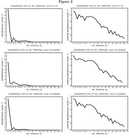
(b) NPL Estimator (Global search): The NPL ﬁxed point associated with the initial frequency

estimator is consistent. However, it is not necessarily the NPL estimator because there may be

other NPL ﬁxed points with higher value of the pseudo likelihood function. We have implemented

the NPL algorithm for diﬀerent values of the initial P₀_{: e.g.,} P₀ _{= 0}_.₅ _{for every market, player}

and state; P₀ _{= 0}_._0000001 _{for every market, player and state;} P₀ _{= 0}_.₉₉₉₉₉₉ _{for every market,}

player and state; and P₀ ₌_{vector of random draws from} _{U nif orm}₍₀_,₁₎_{. In this application, and}

(21)

convergence path is quite similar in all the cases we have tried. Figure 2 presents the convergence

paths for three cases: P₀ _{= 0}_.₅_,P₀_{= 0}_._0000001_{, and} P₀ _{= 0}_.₉₉₉₉₉₉_.

[image:21.612.89.516.132.588.2]

Figure 2

Note that convergence to the NPLﬁxed point is quite slow. In fact, as shown by theﬁgures in

logarithms, the rate of convergence declines when we approach to the NPLﬁxed point. Regardless

the vector of CCPs that we use to initialize the NPL algorithm, 15 NPL iterations or less take us

very close to an NPL ﬁxed point. However, it takes other 15 iterations to really converge to that

ﬁxed point. The convergence criterion that we use ismaxj|ˆθ K j −ˆθ

K−1

(22)

relax that convergence criterion. Alternatively, it is possible to use "accelerate NPL iterations" as

proposed by Kasahara and Shimotsu (2008). For instance, we can apply more than one iteration

in the best response mapping at each NPL iteration. Iterations in the best response mapping are

computationally costly, but this additional cost might be compensated by a smaller number of NPL

iterations.

(c) Comparing Two-Step and NPL estimators. In this application, we ﬁnd important diﬀerences between the parameter estimates using two-step and NPL methods. Figures 3 presents the

esti-mated variables proﬁt functions andﬁxed cost functions for BK and MD under the two estimation

(23)

Appendix: Gauss code

// ********************************************************************* // NPL_DYNAGAME_150909.prg

//

// THIS PROGRAM ESTIMATES A DYNAMIC GAME OF ENTRY-EXIT USING // THE NESTED PSEUDO LIKELIHOOD (NPL) METHOD, AND ACTUAL DATA // ON MCDONALDS AND BURGER KING LOCATION OF OUTLETS IN UK //

// by VICTOR AGUIRREGABIRIA //

// SEPTEMBER 2009 //

// ********************************************************************* //

// SPECIFICATION OF ONE-PERIOD PROFIT FUNCTION // The profit function for firm i is:

//

// Ui = zi(ai,aj) * thetai - ai * epsi //

// where ai is the new entry decision of firm i, aj is the // new entry decision of firm j, zi(ai,aj) are vectors

// of variables, and thetai is a vector of parameters. More specifically, //

// thetai = (VP0i, VP1i, VP2i, FC1i, FC2i) //

// where VP0i, VP1i, and VP2i are parameters in the variable profit function, // FC1i and FC2i are parameters in fixed costs. And

//

// zi(ai,aj) = { S * 1(xi + ai > 0) } // ~{ S * (xi + ai - xj - aj) }

// ~{ S * (xi + ai - xj - aj)^2 } // ~{ -1(xi + ai > 0) }

// ~{ -(xi + ai) } // ~{ -(xi + ai)^2 } //

new ; closeall ;

library pgraph gauss ; format /mb1 /ros 16,4 ;

// **************************************** // PART 1: SPECIFICATION OF SOME CONSTANTS // **************************************** // Constants of the datafile

// Name and address of data file filedat =

"c:\\mypapers\\arvind_rationalizability\\data\\toivanen_waterson_nolondon_120809.dat";

nobs = 2110 ; // Number of observations in data file nmarket = 422 ; // Number of local markets

nyear = 5 ; // Number of years

nvar = 27 ; // Number of variables in dataset // Constants of the model

(24)

dfact = 0.95 ; // Discount factor maxiter = 50 ;

namesb = namesb1 | namesb2 ; // Calculating some constants vstate = seqa(0,1,maxstore) ;

vstate = (vstate.*.ones(maxstore,1)) ~(ones(maxstore,1).*.vstate) ; // Matrix with all possible values of the state variables

nstate = rows(vstate) ; kp1 = rows(namesb1)/2 ; kp2 = rows(namesb2) ; kparam = rows(namesb) ;

// *************************************************** // PART 2. READING DATA AND CONSTRUCTION OF VARIABLES // *************************************************** open dtin = ^filedat for read varindxi ;

data = readr(dtin,nobs); dtin = close(dtin) ; county_name = data[.,1] ; district_name = data[.,2] ; county_code = data[.,3] ; district_code = data[.,4] ; year = data[.,5] ;

mcd_stock = data[.,6] ; mcd_entry = data[.,7] ; mcd_entdum = data[.,8] ; bk_stock = data[.,9] ; bk_entry = data[.,10] ; bk_entdum = data[.,11] ; district_area = data[.,12] ; population = data[.,13] ; pop_0514 = data[.,14] ; pop_1529 = data[.,15] ; pop_4559 = data[.,16] ; pop_6064 = data[.,17] ; pop_6574 = data[.,18] ; avg_rent = data[.,19] ; ctax = data[.,20] ; ecac = data[.,21] ; ue = data[.,22] ; gdp_pc = data[.,23] ;

dist_bkhq_miles = data[.,24] ; dist_bkhq_minu = data[.,25] ; dist_mdhq_miles = data[.,26] ; dist_mdhq_minu = data[.,27] ; // Construction of variables

x_bk = bk_stock ; // Stock of stores for BK x_md = mcd_stock ; // Stock of stores for MD

(25)

// Market specific mean values of some exogenous explanatory variables marketsize = meanc(reshape(population,nmarket,nyear)’) ;

zmarket = meanc(reshape(density,nmarket,nyear)’) ~meanc(reshape(gdp_pc,nmarket,nyear)’)

~meanc(reshape(avg_rent,nmarket,nyear)’) ~meanc(reshape(ctax,nmarket,nyear)’) ; // *******************

// PART 3. PROCEDURES // *******************

// ---// A. PROCEDURE for FREQUENCY ESTIMATOR // ---proc (1) = freqprob(yobs,xobs,xval) ;

// ---// FREQPROB.SRC Procedure that obtains a frequency estimation

// of Prob(Y|X) where Y is a vector of binary

// variables and X is a vector of discrete variables // FORMAT:

// freqp = freqprob(yobs,xobs,xval) // INPUTS:

// yobs - (nobs x q) vector with sample observations // of Y = Y1 ~Y2 ~... ~Yq

//

// xobs - (nobs x k) matrix with sample observations of X //

// xval - (numx x k) matrix with the values of X for which // we want to estimate Prob(Y|X).

// OUTPUTS:

// freqp - (numx x q) vector with frequency estimates of // Pr(Y|X) for each value in xval.

// Pr(Y1=1|X) ~Pr(Y2=1|X) ~... ~Pr(Yq=1|X)

// ---local numx, numq, prob1, t, selx, denom, numer ;

numx = rows(xval) ; numq = cols(yobs) ;

prob1 = zeros(numx,numq) ; t=1 ;

do while t<=numx ;

selx = prodc((xobs.==xval[t,.])’) ; denom = sumc(selx) ;

if (denom==0) ;

prob1[t,.] = zeros(1,numq) ; else ;

numer = sumc(selx.*yobs) ; prob1[t,.] = (numer’)./denom ; endif ;

t=t+1 ; endo ;

retp(prob1) ; endp ;

(26)

// ---// MIPROBIT - Estimation of a Probit Model by Maximum Likelihood

// The optimization algorithm is a Newton’s method // with analytical gradient and hessian

//

// FORMAT {best,varest,llike} = miprobit(ydum,x,rest,b0,nombres,out) //

// INPUTS

// ydum - (nobs x 1) vector with observations of the dependent variable // x - (nobs x k) matrix with observations of explanatory variables // associated with the unrestricted parameters

// rest - vector with observations of the sum of the explanatory // variables whose parameters are restricted to be 1

// (Note that the value 1 is without loss of generality // if the variable rest is constructed appropriately)

// b0 - (k x 1) vector with values of parameters to initialized // Newton’s methos

// nombres - (k x 1) vector with names of parameters to estimate // out - 0=no table of results; 1=table with estimation results //

// OUTPUTS

// best - ML estimates

// varest - estimate of the covariance matrix

// llike - value of log-likelihood function at the MLE

// ---local myzero, nobs, nparam, eps, iter, llike,

criter, Fxb0, phixb0, lamdab0, dlogLb0,

d2logLb0, b1, lamda0, lamda1, Avarb, sdb, tstat, numy1, numy0, logL0, LRI, pseudoR2, k ;

myzero = 1e-36 ; nobs = rows(ydum) ; nparam = cols(x) ; eps = 1E-6 ;

iter=1 ;

llike = 1000 ; criter = 1000 ;

do while (criter>eps) ; if (out==1) ;

"" ;

"Pseudo MLE Iteration = " iter ; "Log-Likelihood function = " llike ; "Criterion = " criter ;

"" ; endif ;

Fxb0 = cdfn(x*b0+rest) ;

Fxb0 = Fxb0 + (myzero - Fxb0).*(Fxb0.<myzero) + (1-myzero - Fxb0).*(Fxb0.>(1-myzero));

llike = ydum’*ln(Fxb0) + (1-ydum)’*ln(1-Fxb0) ; phixb0 = pdfn(x*b0+rest) ;

lamdab0 = ydum.*(phixb0./Fxb0) + (1-ydum).*(-phixb0./(1-Fxb0)) ; dlogLb0 = x’*lamdab0 ;

d2logLb0 = -((lamdab0.*(lamdab0 + x*b0 + rest)).*x)’*x ; b1 = b0 - inv(d2logLb0)*dlogLb0 ;

(27)

b0 = b1 ;

iter = iter + 1 ; endo ;

Fxb0 = cdfn(x*b0 + rest) ;

Fxb0 = Fxb0 + (myzero - Fxb0).*(Fxb0.<myzero) + (1-myzero - Fxb0).*(Fxb0.>(1-myzero));

llike = ydum’*ln(Fxb0) + (1-ydum)’*ln(1-Fxb0) ; phixb0 = pdfn(x*b0 + rest) ;

lamda0 = -phixb0./(1-Fxb0) ; lamda1 = phixb0./Fxb0 ;

Avarb = ((lamda0.*lamda1).*x)’*x ; Avarb = inv(-Avarb) ;

sdb = sqrt(diag(Avarb)) ; tstat = b0./sdb ;

numy1 = sumc(ydum) ; numy0 = nobs - numy1 ;

logL0 = numy1*ln(numy1) + numy0*ln(numy0) - nobs*ln(nobs) ; LRI = 1 - llike/logL0 ;

pseudoR2 = 1 - ( (ydum - Fxb0)’*(ydum - Fxb0) )/numy1 ; if (out==1) ;

"Number of Iterations = " iter ; "Log-Likelihood function = " llike ; "Likelihood Ratio Index = " LRI ; "Pseudo-R2 = " pseudoR2 ;

"" ;

"---"; " Parameter Estimate Standard t-ratios";

" Errors" ;

"---"; k=1;

do while k<=nparam;

print $nombres[k];;b0[k];;sdb[k];;tstat[k]; k=k+1 ;

endo;

"---"; endif ;

retp(b0,Avarb,llike) ; endp ;

// ---// C. PROCEDURE for NPL ESTIMATOR //

---proc (4) = npl_bkmd(yobs, xobs, msize, zmarket, pchoice, mstate, beta, kiter, namesb); //

---// NPL_BKMD

// This procedure iterates in the NPL algorithm given an initial vector // of CCPs. The model is the dynamic game of local market entry for

// McDonalds and Burger King. The procedure returns the vector of parameter // estimates, the variance matrix, and the matrix with players choice

// probabilities at every state, and at every sample point. //

// FORMAT (thetaest,varest,pest,pest_obs) =

// npl_bkmd(yobs, xobs, msize, zmarket, pchoice, mstate, beta, kiter, namesb) //

(28)

// yobs - (nobs x 2) matrix with observations of players’ choices // xobs - (nobs x 2) matrix with observations of players’ endogenous // state variables

// msize - (nmarket x 1) vector with observations of market size (population) // zmarket - (nmarket x kz) matrix with observations of time-invariant

// market chracteristics

// pchoice - (nstate*nmarket x 2) matrix with initial vector of CCPs for // every market, state and player

// mstate - (nstate x 2) matrix with all the possible values of the // endogenous state variables

// beta - Scalar with value of the discount factor

// kiter - Scalar natural number with number of NPL iterations // namesb - (K x 1) vector with names of the structural parameters //

// OUTPUTS

// thetaest - (K x1) vector with parameter estimates at the last NPL iteration // varest - (K xK) matrix of variances and covariances

// pest - (nstate*nmarket x 2) matrix with estimates of CCPs for // every market, state and player

// pest_obs - (nobs x 2) matrix with estimates of CCPs for every // observation and state

//

---local myzero, nobs, nmarket, nyear, nplayer, ns, numx, ktot, kvpfc, kz, indxobs, j,

xbk, xmd, npliter, criterion, conv_const, theta0,

p_bk, p_md, ztilda_bk, ztilda_md, etilda_bk, etilda_md, ztilda_obs_bk, ztilda_obs_md, etilda_obs_bk, etilda_obs_md, m, valmsize, valzmarket,

zbk_00, zbk_01, zbk_10, zbk_11, zmd_00, zmd_01, zmd_10, zmd_11, eprofbk_0, eprofbk_1, eprofmd_0, eprofmd_1,

tranxbk_bk0, tranxbk_bk1, tranxmd_md0, tranxmd_md1, tranxmd_bk, tranxbk_md, tottran_bk0, tottran_bk1, tottran_md0, tottran_md1, uncontran,

value_z_bk, value_z_md, value_e_bk, value_e_md, zt_bk, zt_md, et_bk, et_md, count1, count2,

zobs, eobs, thetaest, varest, likelihood, theta_bk, theta_md, pest_obs ; //

---// Some constants //

---myzero = 1e-12 ; // Constant for truncation of CCPs to avoid numerical errors nobs = rows(yobs) ; // Total number of market*year observations

nmarket = rows(msize) ; // Total number of markets in the sample

nyear = nobs/nmarket ; // Number of years in the sample (balanced panel)

if nyear/=int(nyear) ; "ERROR: Number of years is not an integer"; end; endif;

nplayer = cols(yobs) ;

ns = rows(pchoice)/nmarket ; // number of states in a single market

if ns/=int(ns) ; "ERROR: Number of states in a single market is not an integer"; end; endif;

numx = sqrt(ns) ; // number of values of xbk or xmd

if numx/=int(numx) ; "ERROR: Number of values of xbk or xmd is not an integer"; end; endif;

(29)

kz = cols(zmarket) ; // Number of parameters associated with the control variables in zmarket

kvpfc = (ktot-kz)/2 ; // Number of parameters in var profits and fixed costs for a single firm

if kvpfc/=int(kvpfc) ; "ERROR: Number of parameters in var profits and fixed costs is not an integer"; end; endif;

xbk = mstate[.,1] ; // vector stock of stores for BK xmd = mstate[.,2] ; // vector stock of stores for MD //

---// Vector with indexes for the observed state // ---indxobs = zeros(nobs,1) ;

j=1 ;

do while j<=ns ;

indxobs = indxobs + j.*prodc((xobs.==mstate[j,.])’) ; j=j+1 ;

endo ;

// ---// NPL algorithm // ---criterion = 1000 ; conv_const = 1e-6 ; theta0 = zeros(ktot,1) ; npliter=1 ;

do while (npliter<=kiter).and(criterion>conv_const) ; "NPL ITERATION =";; npliter ;; "Criterion =";; criterion ; "" ;

// ---// TASK 1: Computing the matrices ztilda_bk and ztilda_md // and the vectors etilda_bk and etilda_md

// for every market and every sample observation

// ---ztilda_bk = zeros(nmarket*ns,kvpfc+kz) ;

ztilda_md = zeros(nmarket*ns,kvpfc+kz) ; etilda_bk = zeros(nmarket*ns,1) ;

etilda_md = zeros(nmarket*ns,1) ; ztilda_obs_bk = zeros(nobs,kvpfc+kz) ; ztilda_obs_md = zeros(nobs,kvpfc+kz) ; etilda_obs_bk = zeros(nobs,1) ;

etilda_obs_md = zeros(nobs,1) ; m=1;

do while m<=nmarket ; valmsize = msize[m] ;

valzmarket = zmarket[m,.] ;

// ---// Selection of probabilities for the market and

// truncation of probabilities to avoid inverse Mill’s ratio = +INF // ---p_bk = pchoice[(m-1)*ns+1:m*ns,1] ;

p_md = pchoice[(m-1)*ns+1:m*ns,2] ; p_bk = (p_bk.<=myzero).*myzero + (p_bk.>=(1-myzero)).*(1-myzero)

(30)

+ (p_md.>=(1-myzero)).*(1-myzero)

+ (p_md.>=myzero).*(p_md.<=(1-myzero)).*p_md ; //

---// Vectors of expected profits //

---zbk_00 = (valmsize.*(xbk.>0)) ~(valmsize.*(xbk-xmd)) ~(valmsize.*(xbk-xmd).*(xbk-xmd))

~(-(xbk.>0)) ~(-xbk) ~(-xbk.*xbk) ~(valzmarket.*xbk) ;

zbk_01 = (valmsize.*(xbk.>0)) ~(valmsize.*(xbk-xmd-1)) ~(valmsize.*(xbk-xmd-1).*(xbk-xmd-1))

~(-(xbk.>0)) ~(-xbk) ~(-xbk.*xbk) ~(valzmarket.*xbk) ;

zbk_10 = (valmsize.*((xbk+1).>0))~(valmsize.*(xbk+1-xmd)) ~(valmsize.*(xbk+1-xmd).*(xbk+1-xmd))

~(-((xbk+1).>0)) ~(-(xbk+1)) ~(-(xbk+1).*(xbk+1)) ~(valzmarket.*(xbk+1)) ;

zbk_11 = (valmsize.*((xbk+1).>0))~(valmsize.*(xbk+1-xmd-1)) ~(valmsize.*(xbk+1-xmd-1).*(xbk+1-xmd-1))

~(-((xbk+1).>0)) ~(-(xbk+1)) ~(-(xbk+1).*(xbk+1)) ~(valzmarket.*(xbk+1)) ;

zmd_00 = (valmsize.*(xmd.>0)) ~(valmsize.*(xmd-xbk)) ~(valmsize.*(xmd-xbk).*(xmd-xbk))

~(-(xmd.>0)) ~(-xmd) ~(-xmd.*xmd) ~(valzmarket.*xmd) ;

zmd_01 = (valmsize.*(xmd.>0)) ~(valmsize.*(xmd-xbk-1)) ~(valmsize.*(xmd-xbk-1).*(xmd-xbk-1))

~(-(xmd.>0)) ~(-xmd) ~(-xmd.*xmd) ~(valzmarket.*xmd) ;

zmd_10 = (valmsize.*((xmd+1).>0))~(valmsize.*(xmd+1-xbk)) ~(valmsize.*(xmd+1-xbk).*(xmd+1-xbk))

~(-((xmd+1).>0)) ~(-(xmd+1)) ~(-(xmd+1).*(xmd+1)) ~(valzmarket.*(xmd+1)) ;

zmd_11 = (valmsize.*((xmd+1).>0))~(valmsize.*(xmd+1-xbk-1)) ~(valmsize.*(xmd+1-xbk-1).*(xmd+1-xbk-1))

~(-((xmd+1).>0)) ~(-(xmd+1)) ~(-(xmd+1).*(xmd+1)) ~(valzmarket.*(xmd+1)) ;

eprofbk_0 = (1-p_md).*zbk_00 + p_md.*zbk_01 ; // Expected Profit BK if a=0 eprofbk_1 = (1-p_md).*zbk_10 + p_md.*zbk_11 ; // Expected Profit BK if a=1 eprofmd_0 = (1-p_bk).*zmd_00 + p_bk.*zmd_01 ; // Expected Profit MD if a=0 eprofmd_1 = (1-p_bk).*zmd_10 + p_bk.*zmd_11 ; // Expected Profit MD if a=1 //

---// Transition probabilities //

---// Remember: vstate = xbk ~xmd

// where: xbk = (1|2| ... |14).*.(1|1|....|1) // xmd = (1|1| ... |1) .*.(1|2|....|14)

// Transition xbk for BK: abk = 0

// Pr( xbk’ | xbk, xmd, abk =0) = 1{xbk’ = xbk)

tranxbk_bk0 = eye(numx) ; // Transition of xbk in the space of xbk

(31)

// Transition xbk for BK: abk = 1

// Pr( xbk’ | xbk, xmd, abk =0) = 1{xbk’ = xbk+1) tranxbk_bk1 = (zeros(numx-1,1) ~eye(numx-1))

| (zeros(1,numx-1) ~1); // Transition of xbk in the space of xbk

tranxbk_bk1 = tranxbk_bk1.*.ones(numx,numx) ; // Transition of xbk in the space of xbk, xmd

// Transition xmd for MD: amd = 0

// Pr( xmd’ | xbk, xmd, amd =0) = 1{xmd’ = xmd)

tranxmd_md0 = eye(numx) ; // Transition of xmd in the space of xmd

tranxmd_md0 = ones(numx,numx).*.tranxmd_md0 ; // Transition of xmd in the space of xbk, xmd

// Transition xmd for MD: amd = 1

// Pr( xmd’ | xbk, xmd, amd =1) = 1{xmd’ = xmd+1) tranxmd_md1 = (zeros(numx-1,1) ~eye(numx-1))

| (zeros(1,numx-1) ~1); // Transition of xmd in the space of xmd

tranxmd_md1 = ones(numx,numx).*.tranxmd_md1 ; // Transition of xmd in the space of xbk, xmd

// Transition xmd from the point of view of BK who doesn’t know amd // Pr( xmd’ | xbk, xmd) = (1-pmd) * 1{xmd’ = xmd) + pmd * 1{xmd’ = xmd+1) tranxmd_bk = (1-p_md).* tranxmd_md0 + p_md.* tranxmd_md1 ;

// Transition xbk from the point of view of MD who doesn’t know abk // Pr( xbk’ | xbk, xmd) = (1-pbk) * 1{xbk’ = xbk) + pbk * 1{xbk’ = xbk+1) tranxbk_md = (1-p_bk).* tranxbk_bk0 + p_bk.* tranxbk_bk1 ;

// Total transition matrix of (xbk,xmd) for BK if abk = 0

// Pr( xbk’,xmd’ | xbk, xmd, abk=0) = Pr( xbk’ | xbk, abk =0) * Pr( xmd’ | xbk, xmd) tottran_bk0 = tranxbk_bk0 .* tranxmd_bk ;

if sumc(sumc(tottran_bk0’).>(1.00001)) or sumc(sumc(tottran_bk0’).<(0.99999)) ;

"ERROR: Transition matrix does not sum 1" ; end ; endif ;

// Total transition matrix of (xbk,xmd) for BK if abk = 1

// Pr( xbk’,xmd’ | xbk, xmd, abk=1) = Pr( xbk’ | xbk, abk =1) * Pr( xmd’ | xbk, xmd) tottran_bk1 = tranxbk_bk1 .* tranxmd_bk ;

if sumc(sumc(tottran_bk1’).>(1.00001)) or sumc(sumc(tottran_bk1’).<(0.99999)) ;

// Total transition matrix of (xbk,xmd) for MD if amd = 0

// Pr( xbk’,xmd’ | xbk, xmd, amd=0) = Pr( xmd’ | xmd, amd =0) * Pr( xbk’ | xbk, xmd) tottran_md0 = tranxmd_md0 .* tranxbk_md ;

if sumc(sumc(tottran_md0’).>(1.00001)) or sumc(sumc(tottran_md0’).<(0.99999)) ;

// Total transition matrix of (xbk,xmd) for MD if amd = 1

// Pr( xbk’,xmd’ | xbk, xmd, amd=1) = Pr( xmd’ | xmd, amd =1) * Pr( xbk’ | xbk, xmd) tottran_md1 = tranxmd_md1 .* tranxbk_md ;

if sumc(sumc(tottran_md1’).>(1.00001)) or sumc(sumc(tottran_md1’).<(0.99999)) ;

// Unconditional transition matrix

(32)

if sumc(sumc(uncontran’).>(1.00001)) or sumc(sumc(uncontran’).<(0.99999)) ; "ERROR: Transition matrix does not sum 1" ; end ;

endif ;

// ---// ztilda_bk, ztilda_md, etilda_bk, etilda_md for every possible state // ---uncontran = inv(eye(ns) - beta*---uncontran) ; // Matrix (I - beta*F)^-1 value_z_bk = (1-p_bk).*eprofbk_0 + p_bk.*eprofbk_1 ;

value_z_bk = uncontran * value_z_bk ; // Value Z function BK

value_e_bk = uncontran * pdfn(cdfni(p_bk)) ; // Value e function BK value_z_md = (1-p_md).*eprofmd_0 + p_md.*eprofmd_1 ;

value_z_md = uncontran * value_z_md ; // Value Z function MD

value_e_md = uncontran * pdfn(cdfni(p_md)) ; // Value e function MD

zt_bk = (eprofbk_1 - eprofbk_0) + beta*(tottran_bk1-tottran_bk0)*value_z_bk ; zt_md = (eprofmd_1 - eprofmd_0) + beta*(tottran_md1-tottran_md0)*value_z_md ; et_bk = beta*(tottran_bk1-tottran_bk0)*value_e_bk ;

et_md = beta*(tottran_md1-tottran_md0)*value_e_md ; //

---// Filling //

---count1 = (m-1)*ns + 1 ; count2 = m*ns ;

ztilda_bk[count1:count2,.] = zt_bk ; ztilda_md[count1:count2,.] = zt_md ; etilda_bk[count1:count2,.] = et_bk ; etilda_md[count1:count2,.] = et_md ; count1 = (m-1)*nyear + 1 ;

count2 = m*nyear ;

ztilda_obs_bk[count1:count2,.] = zt_bk[indxobs[count1:count2],.] ; ztilda_obs_md[count1:count2,.] = zt_md[indxobs[count1:count2],.] ; etilda_obs_bk[count1:count2,.] = et_bk[indxobs[count1:count2],.] ; etilda_obs_md[count1:count2,.] = et_md[indxobs[count1:count2],.] ;

m=m+1; endo ;

// ---// TASK 2: Pseudo Maximum Likelihood Estimation // ---zobs = (ztilda_obs_bk[.,1:kvpfc] | zeros(nobs,kvpfc)) ~(zeros(nobs,kvpfc) | ztilda_obs_md[.,1:kvpfc])

~(ztilda_obs_bk[.,kvpfc+1:kvpfc+kz] | ztilda_obs_md[.,kvpfc+1:kvpfc+kz]) ; eobs = etilda_obs_bk | etilda_obs_md ;

{thetaest,varest,likelihood}

= miprobit((yobs[.,1]|yobs[.,2]),zobs,eobs,zeros(ktot,1),namesb,1) ; //

---// TASK 3: Updating Conditional Choice Probabilities // ---theta_bk = thetaest[1:kvpfc] | thetaest[2*kvpfc+1:ktot] ;

theta_md = thetaest[kvpfc+1:2*kvpfc] | thetaest[2*kvpfc+1:ktot] ;

pchoice = cdfn(ztilda_bk*theta_bk + etilda_bk) ~cdfn(ztilda_md*theta_md + etilda_md) ;

(33)

//

---criterion = maxc(abs(thetaest-theta0)) ;

theta0 = thetaest ; npliter = npliter+1 ; endo ;

// ---// Observed Conditional Choice Probabilities: //

---pest_obs = cdfn(ztilda_obs_bk * theta_bk + etilda_obs_bk) ~cdfn(ztilda_obs_md * theta_md + etilda_obs_md) ;

retp(thetaest,varest,pchoice,pest_obs) ; endp ;

// *********************************** // PART 4: ESTIMATION OF INITIAL CCPs // *********************************** prob_freq = zeros(nmarket*nstate,nplayer) ; market = 1 ;

do while market<=nmarket ;

count1 = (market-1)*nstate + 1 ; count2 = market*nstate ;

yyy = a_bk[(market-1)*nyear+1:market*nyear] ~a_md[(market-1)*nyear+1:market*nyear] ;

xxx = x_bk[(market-1)*nyear+1:market*nyear] ~x_md[(market-1)*nyear+1:market*nyear] ;

buff = freqprob(yyy,xxx,vstate) ;

prob_freq[count1:count2,.] = freqprob(yyy,xxx,vstate) ; market = market+1 ;

endo ;

// Alternatively, the user could initialize the NPL algorithm using // a vector of constant probabiliies, e.g.,

// prob_freq = (1/2)*ones(nmarket*nstate,nplayer);

// or using random draws from a uniform distribution, e.g., // prob_freq = rndu(nmarket*nstate,nplayer);

// ************************ // PART 5: NPL ESTIMATION // ************************ {best,varb,pstate,pobs} =

(34)

References

[1] Aguirregabiria, V. and C. Alonso-Borrego, 2009, Labor Contracts and Flexibility: Evidence

from a Labor Market Reform in Spain. Manuscript. University of Toronto. Department of

Economics.

[2] Aguirregabiria, V. and C-Y. Ho, 2009, A dynamic oligopoly game of the US airline industry:

Estimation and policy experiments. Manuscript. University of Toronto.

[3] Aguirregabiria, V. and P. Mira, 2002, Swapping the nested ﬁxed point algorithm: A class of

estimators for discrete Markov decision models. Econometrica 70, 1519-1543.

[4] Aguirregabiria, V. and P. Mira, 2007, Sequential estimation of dynamic discrete games.

Econo-metrica 75, 1—53.

[5] Aguirregabiria, V., P. Mira, and H. Roman, 2007, Inter-industry heterogeneity in market

structure and dynamic oligopoly structural models. Manuscript. The University of Toronto.

[6] Besanko, D., and U. Doraszelski (2004): "Capacity Dynamics and Endogenous Asymmetries

in Firm Size,"RAND Journal of Economics,35, 23-49.

[7] Collard-Wexler, A., 2008, Demand Fluctuations in the Ready-Mix Concrete Industry.

Manu-script. New York University.

[8] De Pinto, A., and G. Nelson, 2007, Modelling Deforestation and Land-Use Change: Sparse

Data Environments. Journal of Agricultural Economics. Vol. 58(3), 502 - 516.

[9] De Pinto, A., and G. Nelson, 2009, Land Use Change with Spatially Explicit Data: A Dynamic

Approach. Environmental and Resource Economics. Vol. 43, 209—229.

[10] Ellickson, P. and S. Misra, 2008, Supermarket Pricing Strategies. Marketing Science. Vol.

27(5), 811-828.

(35)

[12] Kano, K., 2006, Menu Costs, Strategic Interactions and Retail Price Movements. Manuscript.

Queen’s University.

[13] Kasahara, H. and K. Shimotsu (2008): "Pseudo-likelihood Estimation and Bootstrap Inference

for Structural Discrete Markov Decision Models,"Journal of Econometrics, 146(1), 92-106.

[14] Lenzo, J., 2008, Market Structure and Proﬁt Complementarity: The Case of SPECT and PET.

Manuscript. Northwestern University. Kellogg School of Management.

[15] Lin, H., 2008, Quality Choice and Market Structure: A Dynamic Analysis of Nursing Home

Oligopolies. Manuscript. Indiana University. Business School.

[16] Lorincz, S., 2005, Persistence Eﬀects in a Dynamic Discrete Choice Model: Application to Low-End Computer Servers. Discussion Papers 2005/10. Institute of Economics Hungarian

Academy of Sciences.

[17] Ryan, S. (2009): "The Costs of Environmental Regulation in a Concentrated Industry,"

Man-uscript, MIT Department of Economics.

[18] Sanchez-Mangas, R., 2002, Pseudo Maximum Likelihood Estimation of a Dynamic Structural

Investment Model. Working Paper 02-62, Statistics and Econometrics Series. Universidad

Car-los III de Madrid.

[19] Suzuki, J., 2008, Land Use Regulation as a Barrier to Entry: Evidence from the Texas Lodging

Industry. Manuscript. Department of Economics. University of Minnesota.

[20] Toivanen, O., and M. Waterson (2005): "Market Structure and Entry: Where’s the Beef?,"

RAND Journal of Economics, 36(3), 680-699.

[21] Tomlin, B., 2009, Exchange Rate Volatility, Plant Turnover and Productivity. Manuscript.

Department of Economics. Boston University.

[22] Walrath, M., 2008, Religion as an Industry: Estimating a Strategic Entry Model for Churches.