A NOVEL EARLY WARNING SYSTEM USING FUZZY MULTIPLE ATTRIBUTE DECISION MAKING ALGORITHM AND METEOROLOGICAL DATA

5303

OPTIMAL CONTROL OF MULTI-CLASS MULTI-SERVER

QUEUEING SYSTEM

1_{ALI MADANKAN,} 2_{ALI DELAVARKHALAFI*}

1,2_{DEPARTMENT of MATHEMATICAL SCIENCE, YAZD UNIVERSITY, YAZD}

E-mail: 1_{[email protected],} 2_{[email protected]}

*Corresponding author

ABSTRACT

We consider Markovian multi-server queues with two class of customers: high and low-priority ones, and presented a framework for a control problem of such queuing system. Most authors have used Brownian control problems (BCP) as formal diffusion limits and also BCPs are used for queuing network control problems too. In this paper, we also suppose formal diffusion limit to control a queuing system where our problem becomes a control problem with the dynamics of Brownian motion. In a related problem, but simpler, a minimum trajectory has been achieved and is provided as the solution of a stochastic differential equation in one dimension and then for a multi-dimensional problem follows.

Keywords: Optimal Control, Brownian Control, Queuing System.

1. INTRODUCTION

In many cases, finding the optimal control policy of a multi-dimensional problem like multi-class multi-server queuing system becomes a Browian control poroblems (BCPs). The BCPs have a reduction to a one-dimensional problem and therefore a cost function possesses a minimum trajectory. Harrison [14] used BCPs as formal diffusion limits to find fundamental of identifying and analyzing the near optimal policies for a multi-class queuing system. Since then, many authors studied fluid and diffusion control problems to provide optimal solutions for the BCPs and also suboptimal policies for the queuing system (see [19]).

The queuing system in this paper is motivated by a cloud computing system, where a in such system there are several virtual machines in the server pool that each of those virtual machines have a particular combination of resources to allocate, and the job classes refer to different type job streams like the work that authors considered in [20]. In the relation to the cloud computing, abandonment intensities are frequently mentioned as key measures of system performance.

In this paper, we analyze queuing systems with multiple class of different customers. Customer abandonment is an important feature in a wide variety of situations that may be encountered in the

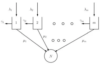
service systems such as cloud computing centers. This paper is also related to the control of a Markovian servicing systems where there is a pool of several servers that serve to different job classes. Figure 1 shows the concern of this paper. In this work, we assume a BCP to formulate a general framework to control a queuing network service. J.M. Harrison and A. Zeevi [16] provided the Hamilton-Jacobi-Bellman (HJB) equation for the BCP to have a unique solution and also M. Armony and C. Maglaras [1] studied the other control problem with the different objective function. In this paper we follow these two work to build a BCP for a single queue and to show that a trajectory solution exists. Then we solve a stochastic differential equation to determine the solution. We also follow the job in the paper [2].

Despite of that The BCPs make available a simplification of the control of queuing system for use, and in compare with the classical method with respect to the convenient, the BCPs may be more difficult to use.

5304 Whitt claimed in [23] that in order to design a system of large-scale services such call centers and allowance customer to abandon, this regime is the best regime to consider.

Some researchers in some research studies has studied and analyzed the control policy of BCPs. Fleming et al [6] used the approximation of this regime to analyze a wireless network, while authors studied the load balancing in [5]. The approximations of performance of a congested communication link is studied in [7]. For systems that consist a large number of servers (e.g., cloud computing [20]), it is appropriate to consider a heavy traffic regime like the one that Halffin and Whitt [10] proposed. Some authors worked on the number of customers in queue and also the number of idle servers and could scale down these parameters by a factor of

N

while time is not scaled (see [15,17,18]).

[image:2.612.318.524.84.241.2]

Our contribution in this paper is the extending multiclass version of the diffusion model. The main contributions are the describing a multi-class generalization in order to the system modeling, and also we consider a finite-horizon cost scale for the diffusion control problem and see that the related Hamilton-Jacobi-Bellman (HJB) equation gives a smooth solution, which is the value function in the sense of mathematical analysis.

[image:2.612.92.290.457.584.2]

Figure 1: A schematic model of the system

Figure 2: A Considered Queuing Model

Let consider that there are

m

different job classes that indicated by

i



1, 2,...,

m

. There is a pool of servers with

N

identical and independent servers, with identical capabilities and resources. Servers are able to serve all jobs from any given class, and we consider that the service intensity



_i depends on the each class

i

that is being processed. We consider that jobs of each class arrive to the system at arrival intensity of



_i and each of them needs a single service before they depart. We also allow customers to abandon the system when they wait in the queue. We consider that abandonment occurs with abandonment intensity



_i (per customer) for class

i

.

We define the quantity c

( )

Q

L

t

related to the BCPs which is the weighted average queue length

by c

( )

i

( )

Q i Q

i

L

t







L

t

, where i

( )

Q

L

t

are the

number of jobs of class

i

in the queue at time

t

. Note that c

( )

Q

L

t

does not meet its minimum trajectory, and specially, minimizing different functionals of c

( )

Q

L

t

may increase to different optimizing policies.

In this paper we want to present that the quantity corresponding to c

( )

Q

5305 classes. In the considered model, customers are able to quit from queue.

2. PROBLEM DEFINITION

WE consider two different classes of jobs and model the problem. The queuing system that we considered is shown in Fig. 2. We consider that it is Poisson arrivals and exponential services. In this paper, we restrict ourselves to 2 classes to ease of computation and formulation, that is, the system under consideration is a multi-class queue with arrival rates of



i

;

i



1, 2

to each queues and abandonment rates



i from queue

i

. Also, we consider that there are finite number,

N

, of identical servers in the server pool that serve to classes with the service rate



_iregarding to class

i

of costumers. Also we consider that there is a dynamic manager in the service pool that schedules the servers to the incoming jobs.

We define two quantities i0

,

i1

Q Q

L

L

to show the queue length of the class

i

and the number of jobs of class

i

where are under service, respectively. With regards to the definition of these quantities, the number of costumer of class

i

in the system

is i i0 i1

Q Q Q

L



L



L

. Let show the arrival process and the potential of service completion by

A t

i

( )

and

P t

i

( )

, respectively, of class

i

until time

t

. Similarly, we define a Poisson process

B t

i

( )

with the abandon rate of



_i, to count abandonments of queue

i

in the considered system. Note that the processes of arrival process, the potential of service completion and abandonments of queue of each classes are independent. By the definition of ij

Q

L

1, 2

i



,

j



0,1

, they are the variables that we define the state of system by them. In case of the any non-idling policy, we do have three variables

10 11

Q Q

L



L

,

L

_Q20 and

L

_Q21.

In this paper, following Bell and Williams [3], the process





( ; )

 

_{1 2} is considered where



_i

( )

t

is the time dedicated to the class

i

until time

t

, totaled on all servers, so the control policy and the process



are related. Note that the processes



_i

( )

t

are constant or increasing processes. By this notations and their definition, one can represent the number of class-

i

served jobs through a server

until time



_i

( )

t

by

P

_i

( ( ))



_i

t

for

i



1;2

. Also this is equal to the number of jobs of class-

i

that one unit server has completed their service until time

t

. Similarly, we consider

W t

_i

( )

be the dedicated waiting time of jobs in all classes until time

t

, where it can be expressed as an integral until time

t

of the variable i0

,

Q

L

and in addition

( ( ))

i i

t

B W

gives us the amount of abandonments jobs from class

i

until time

t

.

We have some restriction that our variables for

1, 2

i



and

j



0,1

and

t



0

must meet the following constraints:

11

_{( )}

21

_{( )}

.

( ) 0

Q Q

ij Q

L

t

L

t

N

L

t







That is, the total number of jobs which are being served, are at most equal to the number of servers. And the queue lengths are not negative.

Another quantity that we want to work with is

( )

i Q

L

t

where it is the total number of costumers of class

i

in the system at time

t

which is

( )

( )

i ij

Q Q

j

L

t





L

t

. The other quantity that we used it to show the sum of idling time of all servers until time

t

, is

L t

( )

. The other set of constraints with derivative of



,

W

and

L

is

1

0

1

,

,

.

i

i Q

i

i Q

i Q i

L

L

L

N

L

W







 









Regarding to the considered quantities, for

i



1, 2

we also have following equations:

0

1 2

( )

( )

(0)

( ( ))

( ( )),

( )

( )

( ),

(1)

( )

( ( )

( )).

i i

Q i Q i i

i i t

i

i Q i

L

t

A t

L

B W t

P

t

t

L

s ds

t

L t

t

W

Nt

t



























5306 By the fact that



_i,

W

_i,

L

for

i



1, 2

are non-decreasing, our constraints are completely described. Since our system has

N

server we consider a sequential system by the number of servers where the number of servers in the

N

th system is

N

. As a result, at each step, the parameters of the sequential systems depend on

N

, where they behave as follow:

,

,

.

N i i N i i N i i

N



















Here to ease of computing we consider the case that

,

N

i

N

i







N

i i







and N

i i







, where by this simplification, one can represent the heavy traffic assumption

(

₁N ₂N

)

/

1

N









as

N

 

by the form of

1 1

1.

(2)

 





Where



_i



 

_i

/

_iand _{i i}

/

N i

N N









Now we define the scaled processes by the following equations:

( )

( ) / ,

( )

( ) / ,

( )

( ) /

,

ˆ ( )

( ) /

,

ˆ ( ) ( ( )

) /

,

( ) (

( )

) /

,

( ) (

( )

) /

,

ˆ

_{( ) (}

_{( )}

₍₀₎

ˆ

ˆ

ˆ

) /

.

N N i N N i N N i i N N N N

i i i

N N

i i i

N N

i i i

i N iN iN

Q Q Q

t

t

N

t

W

t

N

t

W

t

N

L t

L t

N

A

t

A

t

N t

N

t

P

Nt

N

t

N

t

B

Nt

N t

N

L

t

L

t

L

N

W

W

P

B



































Also by considering





*

1 2

( )

t

t

,

t

,





 

and having the processes for

i



1, 2

*

ˆ ( )

N

( ( )

N

( )),

i i i

Y

t



N



t





t

ˆ

ˆ

N

_{( )}

N

ˆ

N

₍

N

_{( ))}

ˆ

N

₍

N

_{( )),}

i i i i i i

X

t



A



B

W

t



P



t

and by assumption the initial condition

ˆ (0) 0

N

i

X



, to have homogenized quantities, we have the following equations:

0

1 2

ˆ

_{( )}

ˆ

_{( )}

ˆ

_{( )}

ˆ

ˆ

ˆ

ˆ

ˆ

( )

( )

( ),

ˆ

_{( )}

ˆ

_{( ).}

iN N N N

Q i i i i i

t

N iN N

i Q i

N N N

L

t

X

t

Y

t

t

L

s ds Y

t

Y

W

W

Y

t

L

t





















The assumption that



N





*

is valid when we consider



N

is given by



*, while the control problem makes a connection to the family of queuing network control problems. Now, the processes

ˆ

N

i

A

,

ˆ

N N

i i

P

_



and, respectively,

ˆ

N N

i i

B

_

W

converge to the mean 0 Brownian motions (BM) with standard derivations

i



,



_i and, respectively, 0.

From this point we are allowed to consider the BCP for the considered problem. Since we are interested with trajectory solutions, we consider the arbitrary costs for our system. Let

X



be independent BM with variances

2 ,



i for

1, 2

i



. By using a control process

( , ,

Y Y W W

_{1 2 1}

,

₂

)

, we need to minimize one of following objectives:

1 1 2

1 2

lim

(

Q

( )

Q

( )),

t

t



L

t



L

t







Or

1 2

1 2

0

(

( )

( )) ,

t

Q Q

E



 

e





L

t





L

t dt

5307 0

1 2

( )

( )

( )

( ),

( )

( )

( ),

(3)

( )

( )

( ),

i

Q i i i i i

i

i Q i

L

t

X t

t

Y t

W t

L

s ds Y t

L t

Y t

W

Y t























where

W

_i and

L

are non-decreasing.

3. CONTROL PROBLEM IN

ONE-DIMENSION

Many other have studied One-dimensional control problem (see [12,13]). Among them Harrison, in [7], with regards to the classical heavy traffic scaling, defined a one dimensional BCP, and showed that it has a unique extremum trajectory. In the other cases the extremum is computed as the solution of the one-dimensional Skorohod equation. In this section, we use optimal control in order to have a unique minimizer trajectory and so its solution that can be found as the solution of some differential equation. The such equation that is used to find the minimum is

( )

( )

( )

,

(0)

(0),

Q Q Q

Q

dL t

dX t

L

t dt

L dt

L

X

















where the notation that we used in this equation

mean as







max(0, )



and

max(0,

)





_

_



_{, and where}

X

is the relate to a BM. By using control variables

Y

and

W

,

the one-dimensional BCP is about to find the optimal cost



₁

L

_Q1





₂

L

_Q2 such that

0

( )

( )

( )

( ),

( )

( )

( ),

(4)

(0)

(0) 0,

Q

t Q

L t

X t

Y t

W t

L s ds

W t

Y t

Y

W





















and

Y

and

W

are non-decreasing.

Theorem 1. Consider Eq. 4 and suppose

 



. Then there exists only one solution for Eq. 4 such

* * * *

(

L

Q

, ,

Y W

, )

L

, where *

Y

and

W

* are minimal if for any possible solution

( , , , )

L Y W L

Q for Eq. 4 one has

*

( )

W t



W t

( ),

t



0 (5)

and

*

( )

Y t



Y t

( ),

t



0 (6)

Also, the parameter

L

_Q* is computed by the

q

that satisfies in

0 0

( )

( )

t

( )

t

( ) ,

q t



X t







q s ds









q s ds



And control variavles

W

* and

Y

* are computed as

* *

0

* *

0

( )

(

( ))

,

( )

(

( ))

.

t Q

t Q

t

L

s

ds

Y t

L

s

d

W

s





 

 





Remark. There are some result from this theorem that followed:

 If  



then we have multiple solutions.

 In order to the relation between



and



, extremumality of

L

_Q* is valid, that is, if

 



,

*

( )

( ),

0

(8)

Q Q

L t



L

t

t



and if

 



*

( )

( ),

0

(9)

Q Q

L t



L

t

t



5308

 In the case





0

, Halfin and Whitt [6] obtained Eq. (8) as the weak limit of a queuing system. Also authors in [15] used the obtained result of [6] to study the abandonment.

 With respect of the optimal policy, Eqs. (8) and (9) express that the summed waiting time and the summed idle time are minimum amount. These equations also show that if

L

Q



0

then

dY



0

and if

0

Q

L



then

dW



0

in the same condition. This, in fact, together with Eq. 4 characterizes the solution

(

L

_Q*

, ,

Y W

* *

)

.

Proof. The functions

L

Q*

, ,

Y W

* * and *

L

are well defined because

x

 is Lipschitz in

X

, and also (8) has a unique solution. With regards to the Eq. 4 and Eq. 7 and as a result of them, one can see the connections between parameters

Y W

*

,

* and

L

_Q*

in the Eq. 9 and Eq. 10. We begin the proof with considering the case

 



. We must prove that:

*

( )

L t

_Q



L

_Q

( ),

t

t



0 (10)

If

( , , , )

L Y W L

_Q satisfies in Eq. 4 then Eq. 5 and Eq. 7 are valid. We declare that the following



( )

t

is non-decreasing

0

( )

t

W t

( )

t

L

Q

( ) .

s ds

(11)



_

_





With respect to the Eq. 4 one can see that both parameters

W t

( )

and

Y t

( )

are non-decreasing.

Where

0

( )

( )

t _Q

( )

Y t



W t





L s ds

. Therefore for

0

 

s

t

one can easily find:

0

0 0

0 0

( )

( )

( )

1

1

1

1

0,

(12)

Q Q

Q Q

t Q

t t

L L

s s

t t

L L

s s

W t

W s

L

d

d

d

dY

dW

 







 

 

























Where the equality holds since integrands are greater than or equal zero and also because of the fact of monotonicity of the integrators. Also from the fact that

s



t

are arbitrary, Eq. 12 holds. With regards to the second equality of Eq. 4, one can see

. .

0 Q 0 Q

,

W

L ds

Y

L ds



_

_



_{ }







By the first equality of Eq. 4, one can see

0

0

( )

( )

( )

( )

(

) ( ).

t

Q Q

t Q

L t

X t

L

s ds

L

s ds

t





  



















If

 





is increasing or constant with initial condition



(0)







(0)

and also if

L L

Q

( )



Q represents the solution associated with



(respectively,





) then

L



_Q



L

_Q (see [4]). Now, we can infer that the solution of this last equation is monotone in



.

Next, with regards to

L

_Q



L

_Q*, we will have that *

(

)

Q Q

L





L

. And therefore from the Eq. 8, we have that

. . _{* *}

0 Q 0

(

Q

)

W





L ds







L



ds



W

Which shows Eq. 5 is valid. Now, with respect to the fist equation of Eq. 4 and also from Eq. 5 and Eq. 10 we have Eq. 7 respectively where it completes the proof when

 



.

Now if

 



, then by substituting



L

_Qinstead of Q

L

and also



X

instead of

X

, swapping

Y

5309 this transformed problem too, and therefore establishes the truth of the original problem that Eq. 5 and Eq. 6 are valid. □

Now, in the following we present a preposition to perform the optimal solution of the control problem.

Proposition. If

 



then the given solution

* * *

(

L

_Q

, ,

Y W

)

of the theorem 1 solves Eq. 4 and also

. 0 0 .

0 0

1

0,

1

0.

(14)

Q Q

L

L

dY

dW













Proof. From theorem 1 we got that

(

L

Q*

, ,

Y W

* *

)

is solution of Eq. 4 and Eq.14. Now let consider

( , , )

L Y W

Q satisfy in the both Eq. 4 and Eq. 14. Then from Eq. 12, for all

t



s

we have

0

( )

( )

1

,

( )

( ) 0.

Q

t L s

t

s

dY

t

s













 







Therefore, we can see that





0

and also

L

_Q

must solve Eq. 7. Since we saw that this equation has only one solution,

L

_Q



L

_Q*

.

If

 



then parameters

U

and

Y

can be presented by the first two equation of Eq. 4 as









. 1

0

. 1

0

(

)

,

(

)

.

Q Q

Q Q

W

L

X

L

Y

L

X

L

 



 











 





 





4. CHARACTERIZATION OF

OPTIMALITY

In this section we consider the standard practice for optimal control and continue with the characterization of the criteria of control problem by using the related Hamilton-Jacobbi-Bellman (HJB) equation. The problem becomes a partial differential equation (PDE) where its solution is the Bellman function

V

. By using the presented state

and control processes, the optimization problem can be wrote as



0



( , )

q

( ( ), ( ( )))

Q Q

J x





E







c L t



L t

dt

Note that

J

(., )



is always well defined functional on the extended positive real number.

Then we have to find the solution of the diffusion control problem by looking for an acceptable policy, by using the following value function which is related to the problem to minimize the functional,

( ) inf (., )

V q

J







If the value function is smooth enough, then it will conduct to the determination of the optimal control policy. Here we present the HJB equation of by (cf. Fleming and Soner 1993,)

2 2

2 1

( )

1

2

( ,

( ))

( ) 0

(15)

m

i i

i i

V x

x

H x

V x

V x





















Here,

:

m m

H





is the Hamiltonian

function:

( , )

inf{ ( , ).

( , ) |

( )}

(16)

H x

b x u

c x u

u

x











U

where

b x u

( , )

is the drift function.

Theorem 1. The HJB Equation (15) has a unique solution and that solution is the value function defined by

( ) inf ( , )

V x

J x







Proof. We organized the proof in several steps. the Because the proof is somewhat lengthy and proceeds in several steps, we first sketch briefly the main ingredients. We begin by applying a standard truncation idea where it helps us to study of PDEs with a Dirichlet boundary condition. We then take a sequence of Dirichlet problems such that the boundary condition vanishes in the limit. The unique solutions to this sequence of truncated

5310 moreover, we show that these functions along with their first and second derivatives constitute an equicontinuous family. Consequently, we can extract a subsequence that converges uniformly on compact sets with the limit being the sought value function which satisfies the original HJB Equation (15).

Step 1. We apply the aforementioned truncation argument, and consider properties of the “truncated

problem.” Fix

n



N

and let

(0, ) { :|| ||

}

B

n



y

y



n

_{. Fix a policy}





_and

an initial condition

X

(0)

 

x

B

(0, )

n

. We will be considering the diffusion

X

_{which solves}

( )

( ( ), ( ( )))

( )

dX t



b X t



X t

dt

 

dW t

“killed” at the boundary of

B

(0, )

n

. Set

inf{

0 : ( )

(0, )

n

T





t



X t



B

n

_{, where for a}

set

S

we let



S

denote its boundary. Where no ambiguity arises, we use

T

n

T

n





_{for brevity. Let}

0

( , )

Tn _t

( ( ), ( ( )))

n x

J x





E





e



c X t



X t

dt

And set

( ) inf

( , )

n n

V x

J x







Fix

r



0

, and set

B

(0, ) { :|| ||

r



y

y



r

}

, the ball of radius

r

_in

R

m_{. Then, for all}

n



[ ] 1

r



_,

we have by the standard interior estimates of Ladyzhenskaya and Uraltseva (1968, pp. 298–300)

that

||



V x

n

( ) ||



C

1 _{for all}

x



B

(0, )

r

_{, where} 1

C

_{is a constant depending on}

_r

_{but independent}

of

n

. A similar estimate holds for

V x

n

( )

_{, which} we make explicit using the following argument. First, note that, and the latter can be bounded using

Fubini’s theorem as follows:

0

( )

_x

[|| ( ) ||]

V x



C





E



X t

dt

for some constant

C

_{independent of}

n

_{. We now have that}

[|| ( ) ||]

(1 || ||)(1

)

x

E



X t



X



x



t

_{. Thus, we}

have

V x

( )



C

2

(1 || ||)



x

_{and this implies the} uniform bound on

V x

n

( )

_.

Step 2. We consider a sequence of truncated problems and their limit. The results stated so far

imply that

{ }

V

n _and

{



V

n

}

_{are bounded} uniformly on compact sets, independent of

n

.

Because

V

n _{satisfies the HJB equation associated} with the truncated problem, and the Hamiltonian is

Lipschitz, it follows that

{





V

n

}

_{is also bounded} on compact sets, independent of

n

. Here





(.)

denotes the second-order operator in the HJB equation, that is, the Laplacian operator, with

weights

2

_,

_{1, 2,}

_n

_{, .}

i

i

m





_Because

{



_

V

_n

}

_and

{



V

n

}

_{are uniformly bounded on}

B

(0, )

r

_{, it} follows that both

V

n _and



V

n _{are Hölder} continuous, in the ball

B

(0, )

r

, uniformly in

n

. Again, because the Hamiltonian is Lipschitz in its

arguments, and because

V

n _{satisfies the PDE with} boundary conditions, it must be that

{





V

n

}

_is also Hölder continuous uniformly in

n

. Hence, the

families

{ }

V

n _,

{



V

n

}

_{, and}

{





V

n

}

_are equicontinuous and bounded. Standard results concerning interchange of derivatives and limits establish the existence of a

V



C

1 such that

n

V



V

_,





V

n

 



V

_{, and}

  

V

n

V

uniformly on

B

(0, )

r

. Standard PDE arguments then give the improved smoothness of

V

. Now,

V

n satisfies the HJB equation with boundary condition

and

V

n



V

_{uniformly on}

B

(0, )

r

_{. Because the} Hamiltonian (16) is Lipschitz, we can “pass” the above limits “through” the truncated HJB equation to establish that

V

satisfies the original HJB PDE on

B

(0, )

r

. Because

r

_{was arbitrary,}

V

_must

5311 that by definition of

V

n _and

V

_{, monotone} convergence implies

0

( )

( ) inf

t

( ( ), ( ( )))

n x

V x

V x

E



e



c X t

X t

dt





  





_

Thus, the proposed limit

V

is the value function of the original control problem. That

V

is finite for all

x

follows from the bound established above, namely,

V x

( )



C

(1 || ||)



x

.

Step 3. The main task here is to apply a verification argument for functions in the class

C

2. Fix

2

W



C

_{, and a policy}





_{. Now, application}

of the Itô differential rule to

exp(





t W X t

) ( ( ))

gives

( )

( , )

lim

inf

t

[ ( ( ))]

(17

)

x t

W x

J x



e



E W X t









Consequently, using

W x

( )



C

(1 || ||)



x

, we have that the last term on the right side of (17) converges to zero. Thus, we have

( )

( , )

W x



J x



_{, and because}



_

_was

arbitrarily chosen, we have

W x

( )



V x

( )

where

V

_{is the value function. On the other hand, the}

optimal policy



* satisfies

*

_{( ())}

_argmin

_{{ ( ( ), ). ( ( )) ( (), ):}

_{( ())}}

X t

b xt u W X t

x X t u u U X t











almost surely for all

t

. Applying Itô’s differential rule as before, we have that

W x

( )



J x

( ,



*

)

. Thus,

W x

( )



V x

( )

, and together with the previous bound establishes that

W

is the value function and



* is an optimal policy. This concludes the proof.

Remark. Let

C

2

(

m

)

denote the class of functions which are twice continuously differentiable over

C

2. Then the HJB Equation has

a unique solution in

C

2, and that solution is the value function.

Proof. See [16].

5. REDUCTION THE DIMENSION

In this section we want to show that we can reduce the dimension of a problem. To do that we need some special consideration on the parameters and then we are able to find minimum trajectory for

1 2

1 2

c

Q Q Q

L





L





L

. We suppose

1 2 1 2

,

 







 

 





without losing generality we can consider

1 2

 



. Also let the processes

L



_Q



L

_Q1



L

_Q2,

1 2

X





X



X

and

W





W

₁



W

₂. Write 1

1 2 2

(

)

( )

( ).

c

Q Q Q

L



 



L

t





L t



By a control that we have for trajectory minimality of

L

_Q1 and

L



_Q, we can find trajectory minimality for c

Q

L

. With regarding to the statement of the BCP Eq. 3 we have following equations:

0

( )

( ),

( )

( ),

,

.

Q t

Q

L

X

I t

W t

W

L s ds

L t

W L are non decreasing































Theorem 1 (see also remark), under the conditions of Eq. 15, gives us the existence of the minimal trajectory

Q



where one can find it as the solution of the following equation

0

( )

0

( ) ,

t t

Q





X









Q s ds











Q s ds





where

W



and

L

are presented by

0

0

( )

( ( ))

,

( )

( ( ))

.

t Q

t Q

W t

L s

ds

L t

L s

ds

















5312 It is notable that the constraints that is expressed in Eq. 14 is a subset of the constraints in Eq. 3. Therefore, if we are able to find the parameters

1

,

2

, ,

Y

1 2

W W

Y

that solve Eq. 3, meanwhile we have

1 2

W



W



W



,

Y

₁



Y

₂



L

, where

W



and

L

are defined in Eq. 18, then we have Eq. 17 as a minimal trajectory

L



_Q for Eq. 3. Now if we consider that

W t

₁

( ) 0



then, parameters

W

₁ and

2

W



W



and

L

satisfy in the non-decreasing constraint. Therefore all constraints of Eq. 3 are held, and

L



_Q from Eq.17 is the minimal of Eq. 3. To check the minimality of

L

_Q1, with regards to

the Eq. 4, we have

L

_Q1from following equation:

1 1

1 ₀

( )

( )

t

( )

( ),

(21)

Q Q

L

t



X t







L

s ds





t

where ₁

0

( ) (

t

)

t

W

( )

s

ds

0





 







for all

t

.

Now, since the solution of Eq. 21 is monotone with respect to the



and since

W

₁



0

,

L

_Q1 is minimized. Hence,

L

_Q1is minimal, and also from

minimality of

L



_Q, we have that c Q

L

is minimal.

6. NUMERICAL SOLUTION

By the analytical characterization of the problem, the objective is to compute it. In this section we follow our assumption of two-class queuing system and try to find the optimal policy numerically.

In order to the numerical example, we consider a queuing system with two different jobs classes with the following parameters: the service rates



₁



1

and



₂



1.5

; the abandonment rates



₁



0.5

and



₂



1

. Now we define

1 2 2 2 2 2 1 2

1 1 1 1 1 2

( , )

(

) ( , )

(

) ( , )

q q

q q

q q



  























We call it “test quantity” and it determines the optimal control. In the definition of the



,



_iis the

i

th element of the gradient vector of the value function and



₁



0.5

and



₂



3

.

The test function  works as follow:

 If

q

₁



q

₂



0

and



( , ) 0

q q

_{1 2}



, then class 1 has the right priority and so the policy works like



₁

( , )

q q

_{1 2}



q

₁ and

2

( , )

q q

1 2

q

1



 

 If and



( , ) 0

q q

_{1 2}



, then class 2 the right priority and so the policy works like

1

( , )

q q

1 2

q

2



 

and



₂

( , )

q q

_{1 2}



q

₂  If

q

₁



q

₂



0

, then all servers in the

server pool are idle and system does not use its capacity

7. CONCLUSION

In this paper we discussed Browian control problem to find optimal control policy in lass multi-server queuing system. The definition of the queuing system is quite general and allows for correlation among the arriving quantities of different job classes. To ease of using notation and also formulation we consider a queuing system only with two classes where our model can be applied to any arbitrary number of classes and we build the parameters by considering a sequence of server. We formulated the problem of finding optimal control policy of a multi-class multi-server queuing system as a Browian control problem and then presented the solution of one dimensional control problem in section 3. Then in the section 4 we showed how to reduce the dimension of the problem to one to solve and to find optimal control for the Browian control problem. The author are suggesting and thinking to study the Browian control problem in the other regime of heavy traffic approximation and also considering a time dependent arrival intensity.

REFERENCES:

[1] M. Armony, C. Maglaras, “Customer contact centers with multiple service channels”, Operations Research, Vol. 52, No. 2, March–April 2004, pp. 271–292. [2] R. Atar, A. Mandelbaum, M. Reiman,

”Scheduling a multi-class queue with many exponential servers: asymptotic optimality in heavy-traffic”, Ann. Appl. Probab., 2004, Vol. 14, No. 3, 1084-1134. [3] S.L. Bell, R.J. Williams, “Dynamic

5313 a continuous review threshold policy”, Ann. Appl. Probab. 11 (3) (2001) 608-649. [4] G. Birkho, G.-C. Rota, “Ordinary Differential Equations”, 4th Edition, Wiley, New York, 1989.

[5] Fleming, P., B. Simon, “Heavy traffic approximations for a system of infinite servers with load balancing”, Probab. Engrg. Inform. Sci. 1999 (13) 251-273. [6] Fleming, P., A. Stolyar, B. Simon, “

Heavy traffic limit for a mobile phone system loss model”, Proc. Nashville ACM Telecomm. Conf., Nashville, TN, 1995. [7] Das, A., R. Srikant, “Diffusion

approximations for a single node accessed by congestion controlled sources”, IEEE Trans. Automatic Control, 2000, 45 1783-1799.

[8] Fleming, W. H., H. M. Soner, “Controlled Markov Processes and Viscosity Solutions”, Applications of Mathematics, Springer-Verlag, Berlin, New York, 1993. [9] O. Garnett, A. Mandelbaum, M. Reiman,

“Designing a call center with impatient

customers”, Manuf. Serv. Oper.

Management 4 (2002) 208-227.

[10]S. Halfin, W. Whitt, “Heavy-traffic limits for queues with many exponential servers”, Oper. Res. 29 (3) (1981) 567-588.

[11]J.M. Harrison, “Brownian Motion and Stochastic Flow Systems”, Wiley Series in Probability and Mathematical Statistics, Wiley, New York, 1985.

[12]V. Dmitruk, A. K. Vdovina, “Study of a one-dimensional optimal control problem with a purely state-dependent cost”, International Conference Stability and Oscillations of Nonlinear Control Systems (Pyatnitskiy's Conference), IEEE conferences, 2016.

[13]K. Papafitsoros, K. Bredies, “A study of the one dimensional total generalised variation regularisation problem”, Inverse Problems and Imaging, 2015, 9: 511–550. [14] J.M. Harrison, “Brownian models of

queuing networks with heterogeneous customer populations”, Stochastic Differential Systems, Stochastic Control Theory and Applications, Springer, New York, 1988, pp. 147-186.

[15]Mandelbaum, W.A. Massey, M. Reiman, B. Rider, A. Stolyar, “Queue length and waiting times for multi-server queues with

abandonment and retrials”, Telecomm. Systems 21 (2–4) (2002) 149-171.

[16]J. M. Harrison, A. Zeevi, “Dynamic scheduling of a multiclass queue in the Halfin–Whitt heavy traffic regime”, Oper. Res.,(2004) 243 - 257.

[17]Mandelbaum, W.A. Massey, M. Reiman, A. Stolyar, “Waiting time asymptotics for the time varying multiserver queue with abandonment and retrials”, 37th Annual Allerton Conference, Allerton, IL, 1999. [18]A.A. Puhalskii, M.I. Reiman, “The

multiclass GI/PH/N queue in the Halfin-Whitt regime”, Adv. in Appl. Probab. 32 (2) (2000) 564-595.

[19]R. J. Williams, “On the approximation of queueing networks in heavy traffic”, in Stochastic Networks: Theory and Applications, Proceedings of Royal Society Workshop, Edinburgh, 1995, F. P. Kelly, S. Zachary, I. Ziedins (eds), Oxford University Press, Oxford, 1996; pp. 35-56. [20]Ali Madankan, Ali Delavarkhalafi,

“Performance Management on Cloud Using Multi Priority Queuing Systems”, Advanced Research on Cloud Computing Design and Applications. IGI Global, 2015. 229-244. doi:10.4018/978-1-4666-8676-2.ch015

[21]Harrison, J. M., “Heavy traffic analysis of a system with parallel servers: Asymptotic optimality of discrete-review policies”, Ann. Appl. Probab. 1998 (8) 822–848. [22]Harrison, J. M., M. J. López., “Heavy

traffic resource pooling in parallel-server systems” QUESTA 1999 (33) 339–368. [23]Whitt, W., “Understanding the efficiency

of multi-server service systems”, Management Sci. 1992 (38) 708–723. [24]Reed, J. (2009). "The G/GI/N queue in the