Implementation And Comparison Of Constructive Heuristics For The Heterogeneous Fleet Vehicle Routing Problem

6958

Implementation And Comparison Of Constructive

Heuristics For The Heterogeneous Fleet Vehicle

Routing Problem

Abstract: The purpose of this article is, firstly, to implement constructive heuristics for the Heterogeneous Fleet Vehicle Routing Problems and secondly, to compare the performance of these heuristics by taking into account the dimension of studied problems, geographical dispersion of served customers, their angular position in relation to the starting point and customer's demand variability. In our study the performance of a solution is calculated in relation to the cost generated by this one, the execution time is not taken into account because constructive heuristics provide generally acceptable solutions in very short time, in the order of a few seconds or even milliseconds, regardless of the problem size.

Index Terms: Vehicle routing problem, CVRP, Heterogeneous Fleet, Constructive Heuristic, Performance Comparison. ——————————  ——————————

1

INTRODUCTION

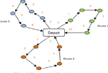
Vehicle routing problems were initially introduced by Dantzig and Ramser [1] in order to solve the distribution problem of fuel to service stations. The basic version of vehicle routing problems, Fig. 1, consists of determining from a depot, the optimal routes to serve a set of customers using a set of vehicles [2].

Fig. 1 Example of vehicle routes

Resolving vehicle routing problems is an important field of operational research and logistics management [3]; these problems are considered NP-hard because they cannot be solved in polynomial time [4]. The evolution of information and communication technologies (ICT) as well as the rise of algorithms, which provides approximate solutions (heuristics) to these problems, has led to a logistic revolution in recent decades. We are interested, in this paper, in constructive heuristics to solve these problems types considering that these heuristics provide acceptable solutions in very short time, with a magnitude order of few seconds or even milliseconds, even face to big dimension problems. The solutions provided by constructive heuristics can also be an entry for another type of more advanced heuristics "metaheuristics" that try to optimize further these solutions.

This article discusses the implementation of constructive heuristics for vehicle routing problem with limited capacity and more generally for the heterogeneous fleet vehicle routing problems. In this article, we compare also these heuristic’s performance through the generation and resolution of a multitude of problems and we determine likewise the parameters that affect the performance of each proposed algorithms. We first begin by introducing the capacitated vehicle routing problems (CVRP), then we expose the heterogeneous fleet vehicle routing problems (HFVRP) and later we detail the principles of the proposed heuristics as well as the implemented algorithms. Secondly, we present the results of performances comparison of the different heuristics for the CVRP problems and for the HFVRP problems by taking into account the number of served customers, geographical dispersion of these customers, their angular position in relation to the starting point and customer's demand variability.

2

VEHICLES

ROUTING

PROBLEMS:

CONCEPTS

AND

EVOLUTIONS

Vehicle routing problems could be modeled as a complete graph G (V, E) where:

V= {v0, v1, v2... vn} is a set of nodes, v0 is the warehouse and the other vi are the destinations to be served by a fleet of m vehicles with a limited capacity Ck.

E= [{vi, vj}, (i, j) ∈ A={(i, j) : i, j=0,1,2, …, n, i ≠j}] is the set of edges connecting the different nodes.

Equations (1) - (5) represents mathematically the vehicle routing problem with limited capacity of vehicles "CVRP" (P1).

∑ ∑ ∑

∑

∑

∈ { }

∑ ∑

∑ ∑

∈ { } _______________________________

• Yassine EL KHAYYAM: PhD student, Laboratory of Industrial Techniques FST-USMBA Fès, Morocco. E-mail: [email protected]

6959 ∑ ∑ ∈ { } ∑ ∑ ∈ | | { }

Equation (1) represents the objective function that minimize necessary costs to serve all customers from warehouse. Cij is the necessary cost to run through the edge (i, j), this one could be the amount of consumed fuel, the consumed time or the traveled distance between i and j. xijk is a binary variable which is equal to 1 if the vehicle k run through the edge (i, j) and 0 if it isn't.

Equation (2) expresses the fact that each vehicle leaving the warehouse to serve one or some customers must return to the warehouse. Equation (3) adds the constraint that node demand must be served once; a single vehicle must serve each node.

Equation (4) ensures that the capacity of each vehicle will not be exceeded. Equation (5) ensures the elimination of sub tours that do not start and / or do not end at the warehouse. The basic version of vehicle routing problem has been transformed into several versions by adding one or more constraints on the initial problem variables. These variables could be the vehicles capacities, the traveled distance, the beginning or arrival time, the delivery or recovery lead-time of the products from warehouse or from customers, there are various types of vehicle routing problems, some of which are below [5].

 MDVRP: this variant takes into consideration several warehouses that can provide products instead of a single warehouse.

 VRPTW: a time window constraint for serving customers is added to the classic vehicle routing problem.

 VRPB deals with two customer’s subgroups, some will have to be delivered from warehouse and the others will forward products to the warehouse.

 OVRP: is to deal with the problems of vehicle routes in which the routes are not closed circuits, the vehicles do not return to the warehouse.

 DVRP: are problems of vehicle routes in which the customer requests are known before (quantities) but can be formulated during the transport operation, these problems are considered dynamic routes problems.  Stochastic VRP [6]: In this VRP variant, no information,

about customer requests, is available before starting routes. Vehicle routes are planned based on probability distributions of customer requests.

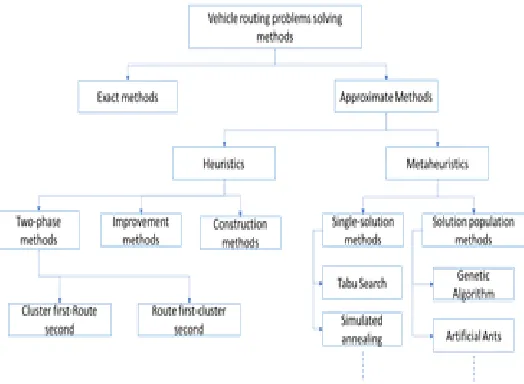
The vehicle routing problem was addressed in the literature by two types of methods [7], Fig. 2, exact methods and approximate methods. The exact methods allow finding the optimal solution by exploring all possible solutions. However, the increase of the studied problem dimension (number of served clients and / or number of logistics means) makes exhaustive exploration of all solutions impossible in a sufficiently small duration.

Fig. 2 VRP resolution methods

The approximate methods, on the other hand, make it possible to find acceptable solutions but do not guarantee that the solution found is the optimal solution. There are two types of approximate methods, heuristics and metaheuristics. Heuristics are by definition a way to guide an algorithm to reduce the problem complexity; they are specific to a given problem. We distinguish three heuristics specific to the vehicle routing problems:

 Constructive heuristics are iterative algorithms in which at each iteration a partial solution is completed. The most popular constructive heuristic is the "savings" heuristic [8], it starts from an initial solution where each destination is served by a vehicle then we try to merge routes by computing for each pair of customers (vi, vj) the savings made by going from vi to vj instead of returning to the warehouse. Savings are then ordered and the corresponding customers to the largest saving are grouped together on the same route.

 The improvement heuristics try to improve a solution by proceeding to exchanges customers within routes. The exchanges could be carried out either within the same route or between customers being part of different routes [9].

 The two-phase methods consist of breaking down the vehicle routing problem into two sub-problems, one relating to the clients clustering and the other relating to determining an optimal route for each subgroup. According to the order in which the sub problems are treated, there are two methods, the Cluster First-Route second method and the Route first- Cluster second method.

Metaheuristics are advanced and powerful heuristics that could be applied to any optimization problem; they are divided into two categories: single-solution or local search metaheuristics and metaheuristic population-based solutions. Among the metaheuristics proposed in the literature, we cite below examples of local search metaheuristics, the simulated annealing and the taboo search, and example of metaheuristic population-based solutions, the evolutionary algorithms [10].

6960 by Glover [11], its principle is based on the mechanism

inspired by human memory. It performs updates to an initial solution during successive iterations; during each iteration, the method constitutes a set of initial solution neighbor's by performing a single elementary movement. Then it evaluates the objective function value corresponding to the different neighbors obtained and substitutes the initial solution by the best solution founded even if the latter is bad than the initial solution, this helps to avoid local minimums. To avoid going back to a solution already obtained in previous iterations, this method uses a list of taboo movements that it avoids when forming the neighborhood, and it inserts in this list the movement corresponding to the solution obtained during each iteration.

 Simulated annealing: this method was inspired by metallurgist’s techniques that are used to obtain a material with well-ordered molecules in solid state; Annealing involves heating a material to a very high temperature and then slowly lowering the temperature. Simulated annealing [12] applies this process to an optimization problem solution; the objective function is assimilated to the material energy that is subsequently minimized by introducing a fictive temperature. For each iteration, a basic modification is performed to the solution, if this modification implies a decrease of the objective function (E≤0) it is accepted, otherwise, it will

be accepted with a probability equal to , T is a constant temperature until reaching the thermodynamic equilibrium. Once the equilibrium is reached, this temperature is reduced and the whole process is repeated until a reduced temperature is reached (cooled system).

 Evolutionary algorithms are inspired by biological evolution of species; genetic algorithms [13] are the most popular evolutionary algorithms. They start from an initial solution population that they try to improve gradually over several generations by applying in a repetitive way the selection and reproduction principles. The selection principle consists to select the most suitable individuals for survival and reproduction (comparing the value of the corresponding objective function for each individual), and the principle of reproduction consists in mixing, recombining and changing (mutation) characteristics of solutions (parents) to form new solutions (descendants) with new potentialities.

3

HETEROGENEOUS

FLEET

VEHICLE

ROUTING

PROBLEMS:

CONCEPTS

AND

IMPLEMENTATION

Capacitated vehicle routing problems modeled in the first section according to problem (P1), equations 1-5, is a special case of the heterogeneous fleet vehicle routing problems in which different types of vehicles are available each one with a different capacity and different costs whether they are fixed costs or costs depending on traveled distances. In the majority of industrial cases, companies are faced with HFVRP as the transport of goods is done through vehicles of different types and different capacities. Among the factors that make HFVRP problems more confronted in the industrial world than the CVRP problems, we cite [14]:

 Customer-specific requirements (dimensional constraints on warehouses).

 Requirements related to the used roads (narrow streets in urban areas, Limits of weight or size on roads in rural areas ...)

 Fleets of vehicles with different capacities allow generally more flexibility and more optimized costs face to demand variability.

 High capacity vehicles generate generally cheaper costs per transported unit.

There are several variants of the HVRP problem according to taking into account or not of vehicles fixed costs and costs depending on traveled distances and depending on the limited or unlimited number of each type of vehicle. [15] distinguishes five variants of the HFVRP problem:

 HVRPFD in which the number of each type of vehicle is limited, the fixed costs related to each type of vehicles are considered as well as the costs depending on travel distances.

 HVRPD, which is similar to the HFVRPD concerning the limitation of vehicles number and taking into account the dependent costs, the difference lies in not taking into account vehicles fixed costs.

 FSMFD in which the number of each type of vehicle is unlimited, the fixed costs related to each type of vehicle are considered as well as the costs depending on travel distances.

 FSMD in which the number of each type of vehicle is unlimited and the fixed costs by vehicle type are not taken into account.

 FSMF in which the number of each type of vehicle is unlimited and the dependent costs by type of vehicles are not taken into account, only the fixed costs are considered.

The formulation of HVRP problem is obtained by taking into account vehicles fixed costs at the objective function, the equation (1) at problem P1 is substituted by the equation (1 ') where Fk is the fixed cost relative to the vehicle k.

∑ ∑ ∑ ∑ ∑

In the case where the number of one or more types of vehicles is limited, another constraint is to be added to the constraints (2) - (5) of the problem (P1):

∑𝒙

𝒎 𝟔

We are interested in the following to the implementation of some constructive heuristics for the HFVRP problem, to be done we introduce the principle used by each heuristic for the resolution of the capacitated vehicle routing problem (CVRP), and then we expose the extension of these principles to be used in the context of the HFVRP problems. Heuristics that fall within the scope of this study are the savings algorithm and the two-phase algorithms: "cluster first route second" and "route first cluster second.

6961 Clarke and Wright [16]. This algorithm is used in cases where

the number of used vehicles is not fixed in advance. The algorithm consists of assigning initially a vehicle to each customer, then computing the savings made by merging routes. Several iterations are executed, for each iteration the algorithm assess the savings that can be realized by all possible mergers (respecting the vehicle's capacity constraint) and then it merges the routes that provide the best economy. This procedure is repeated until no fusion is possible. The savings achieved through the merger of two routes, Fig.3, are computed as follows (7):

𝒆 𝒅 𝒅 𝒅 𝟕

Fig. 3 merger of two routes

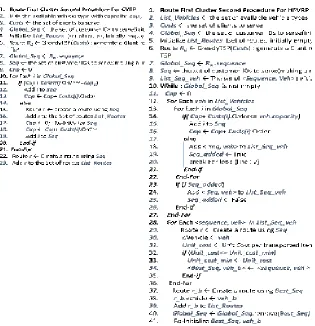
The savings algorithm implemented for the capacitated vehicle routing problems (CVRP) is presented in FIG. 4. In the context of CVRP, distances are used to calculate savings because only one type of transport means is used. However, under the HFVRP, several types of vehicles are available each type has a fixed cost and a distance dependent cost. Savings achieved by merging two routes (a) and (b) using a c-type vehicle (meeting capacity constraints) are calculated using equation (8).

∗ 𝑜𝑠𝑡 ∗ 𝑜𝑠𝑡 ∗ 𝑜𝑠𝑡 𝑜𝑠𝑡 𝑜𝑠𝑡 𝑜𝑠𝑡 8 𝑜𝑠𝑡 : The cost per distance related to the vehicle Va 𝑜𝑠𝑡 : The fixed cost related to the vehicle Va

: The total distance traveled in the route (a)

: The total distance travled in the merged route (ab)

In the case of HFVRP, the merger is performed either by using the vehicle used by one of the two routes or by another vehicle of higher capacity which will allow more interesting savings. Fig. 4 also presents the savings algorithm adapted for HFVRP problems. In each iteration, we determine the best savings that can be obtained by merging two routes and using the different types of available vehicles. As the savings algorithm used for the CVRP, vehicles are initially allocated to each customer, the affected vehicle is the one that generates the least cost.

Fig.4 Savings Algorithm for CVRP and HFVRP

3.2 The "Cluster First Route Second" algorithm for solving CVRP and HFVRP problems

6962

Fig.5 The « sweep » Algorithm

For the second phase, we use greedy algorithms to determine a solution for each TSP problem at each subgroup level.

Greedy algorithms or the Nearest Neighbor algorithms are also considered constructive heuristics for the Travelling Salesman Problem (TSP). It consist in the fact that the sales traveler chooses each time the nearest unvisited customer until he visits all customers and then returns to the depot. FIG. 6 illustrates the algorithms implemented to solve the CVRP problems as well as the HFVRP problems by using the "cluster first route second" approach. The adaptation introduced to the algorithm in order to support the HFVRP is to sweep customers by considering all available vehicle types and for each scenario, the transport cost per unit transported is determined. We select the subgroup, which allows us a minimal unit cost, and then we carry out the same iteration until we constitute all possible SUBGROUPS.

Fig.6 « CFRS » Algorithm for CVRP and HFVRP

3.3 The « Route First Cluster Second » algorithm for solving CVRP and HFVRP problems

Like the algorithm studied in the previous section, the algorithm presented in this paragraph applies in two phases, the first phase is to determine a giant tour regardless of capacities then we cut this giant tour into sub-tours by taking into consideration available vehicle capacities.

The giant tour is determined using the greedy algorithm and then:

 For CVRP problems, we go through the giant route

from the depot until the capacity is exceeded, at the point that precedes the overflow, we go back to the depot to form a tour and we start a new one by starting from the depot to the overflow point. And so on.

6963 is traveled.

FIG. 7 illustrates the algorithms implemented to solve the

CVRP problems as well as the HFVRP problems by using the «route first cluster second " approach.

Fig.7 « RFCS » Algorithm for CVRP and HFVRP

4

COMPARING

CONSTRUCTIVE

HEURISTICS

FOR

CVRP

AND

HVRP

FLEET

VEHICLE

ROUTING

PROBLEMS:

SIMULATIONS

RESULTS

Our objective is comparing the performance of presented heuristics in the previous paragraphs to solve capacitated vehicle routing problems and heterogeneous fleet vehicle routing problems. We have implemented an application to randomly generate both the geographic coordinates of customers and the demand expressed by each customer. We have generated problems in which geographic customer distribution follows a normal law and even problems for which geographic customer distribution follows a uniform law. The input parameters are:

 The number of customers

 The dispersion between customers in the case where the geographic customer’s distribution follows a Normal law (very close points: small dispersion or far points: great dispersion).

 The radial zone to which customers belong according to the depot (points to concentrate between zero and /2 according to the depot or distributed between zero and 2.

 Customer demand compared to available capacities  (customer demand is generated in a uniform random

way between zero and a maximum demand that will be

 variant).

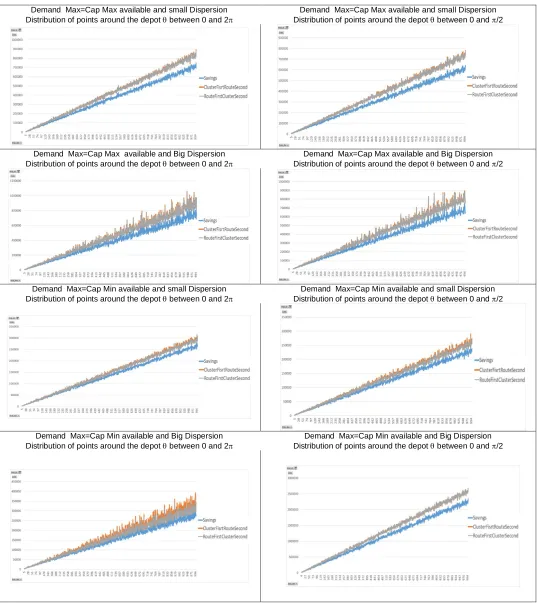
6964 Demand Max=Cap Max available and small Dispersion

Distribution of points around the depot  between 0 and 2

Demand Max=Cap Max available and small Dispersion Distribution of points around the depot  between 0 and /2

Demand Max=Cap Max available and Big Dispersion Distribution of points around the depot  between 0 and 2

Demand Max=Cap Max available and Big Dispersion Distribution of points around the depot  between 0 and /2

Demand Max=Cap Min available and small Dispersion Distribution of points around the depot  between 0 and 2

Demand Max=Cap Min available and small Dispersion Distribution of points around the depot  between 0 and /2

Demand Max=Cap Min available and Big Dispersion Distribution of points around the depot  between 0 and 2

Demand Max=Cap Min available and Big Dispersion Distribution of points around the depot  between 0 and /2

Table 1. Simulation Results for CVRP Problems

In the context of HFVRP problems the performance of the three methods do not depend visibly on the customers dispersion nor on the geographical distribution around the

6965 Demand Max=Cap Max available and small Dispersion

Distribution of points around the depot  between 0 and 2

Demand Max=Cap Max available and small Dispersion Distribution of points around the depot  between 0 and /2

Demand Max=Cap Max available and Big Dispersion Distribution of points around the depot  between 0 and 2

Demand Max=Cap Max available and Big Dispersion Distribution of points around the depot  between 0 and /2

Demand Max=Cap Min available and small Dispersion Distribution of points around the depot  between 0 and 2

Demand Max=Cap Min available and small Dispersion Distribution of points around the depot  between 0 and /2

Demand Max=Cap Min available and Big Dispersion Distribution of points around the depot  between 0 and 2

6966 Table 2. Simulation Results for HFVRP Problems

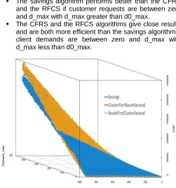
It can be seen that when the maximum demand a customer can express is considerably small compared to the maximum available capacity, the savings method provides worse solutions than those provided by the CFRS method or those provided by the RFCS method in the context of HFVRP. To better visualize this behavior we will vary for each given dimension n, the maximum demand "demand_max" that can express a client (the request is generated randomly between 0 is demand_max) The demand_max parameter is between 0 and the maximum available capacity (the biggest capacity available of available vehicles ). The results obtained are plotted in FIG. 8, which shows that there is a certain value d0_max less than the maximum capacity of available vehicles for which:

 The savings algorithm performs better than the CFRS and the RFCS if customer requests are between zero and d_max with d_max greater than d0_max.

 The CFRS and the RFCS algorithms give close results and are both more efficient than the savings algorithm if client demands are between zero and d_max with d_max less than d0_max.

Fig.8 the evolution of costs according to problem size and

maximum allowed demand

4

CONCLUSION

We have implemented in this article some constructive heuristics to solve capacitated vehicle routing problems then we adapted these heuristics to solve heterogeneous fleet vehicle routing problems. We have implemented an application that allows on one hand to generate problems by taking into account the number of customers to serve, the dispersion between customers, their positioning according to the depot and the maximum demand expressed by each customer. On the other hand, the developed application makes it possible to provide and qualify performance of the different solutions obtained by each heuristic for a given problem. Following a multitude of simulations (thousands) that we have carried out for both types of problems, we have found that for the CVRP problem, the savings algorithm is more efficient than the "cluster first route second" algorithm and "route first cluster

second" algorithm (as implemented) regardless of any parameters that was involved. On the other side, we have found that for HFVRP problems; When the maximum demand that customers could express is considerably small compared to the maximum available capacity, the savings method provides solutions that are not as good as those provided by the other two methods. Reciprocally, when the maximum customers demand is close to the maximum available capacity.

REFERENCES

[1]. R. Dantzig, J. Ramzer (1959). The truck-dispatching problem. Management Science 6(1):81–91

[2]. A.O. Adewumi & O.J. Adeleke, A survey of recent advances in vehicle routing problems, International Journal of System Assurance Engineering and

Management (2018) 9: 155.

https://doi.org/10.1007/s13198-016-0493-4

[3]. C. Wujun, Y. Wenshui (2017), A Survey of Vehicle Routing Problem, MATEC Web of Conferences 100, 0100.

[4]. JK. Lenstra, AHG. Rinnooy Kan (1981) Complexity of vehicle routing and scheduling problems. Networks 11(2):221–227.

[5]. Dixit, & A. Mishra & A. Shukla, (2019). Vehicle Routing Problem with Time Windows Using Meta-Heuristic Algorithms: A Survey: Theory and Applications, ICHSA 2018. 10.1007/978-981-13-0761-4_52.

[6]. R. Maini & R. Goel, (2017). Vehicle routing problem and its solution methodologies: a survey. International Journal of Logistics Systems and

Management. 28. 419.

10.1504/IJLSM.2017.10008188.

[7]. B.I. Sahbi et al (2011), Synthèse du problème de routage de véhicules, Collection des rapports de recherche de Telecom Bretagne.

[8]. G.Clarke and JW Wright. Scheduling of vehicles from a central depot to a number of delivery points. Operations research, 12(4) :568-581, 1964.

[9]. T.G. Crainic and F. Semet. Recherche opérationnelle et transport de marchandises. In Optimisation combinatoire. 3, Applications. Hermès Science: Lavoisier, 2006.

[10]. P. Siarry (ed.), Metaheuristics, Springer International Publishing Switzerland 2016, DOI 10.1007/978-3-319-45403-0_1.

[11]. Glover, F.: Future paths for integer programming and links to artificial intelligence. Computers and Operations Research 13(5), 533–549 (1986). [12]. Kirkpatrick, S., Gelatt, C., Vecchi, M.: Optimization

by simulated annealing. Science 220(4598), 671– 680 (1983)

[13]. Goldberg, D.E.: Genetic Algorithms in Search, Optimization and Machine Learning. Addison- Wesley (1989)

6967 composition and routing. Computers & Operations

Research. 37. 2041-2061.

10.1016/j.cor.2010.03.015.

[15]. Baldacci, Roberto & Battarra, Maria & Vigo, Daniele. (2008). Routing a Heterogeneous Fleet of Vehicles. 10.1007/978-0-387-77778-8_1.

[16]. G. Clarke and J. Wright ―Scheduling of vehicles from a central depot to a number of delivery points‖, Operations Research, 12 #4, 568-581, 1964