A Numerical Study of the Limiting Cases of Cylinder-Induced Shock Wave/Boundary Layer Interactions

(1)

University of Tennessee, Knoxville

Trace: Tennessee Research and Creative

Exchange

Masters Theses Graduate School

5-2017

A Numerical Study of the Limiting Cases of

Cylinder-Induced Shock Wave/Boundary Layer

Interactions

Stefen Albert Lindorfer

University of Tennessee, Knoxville, [email protected]

This Thesis is brought to you for free and open access by the Graduate School at Trace: Tennessee Research and Creative Exchange. It has been Recommended Citation

Lindorfer, Stefen Albert, "A Numerical Study of the Limiting Cases of Cylinder-Induced Shock Wave/Boundary Layer Interactions. " Master's Thesis, University of Tennessee, 2017.

(2)

To the Graduate Council:

I am submitting herewith a thesis written by Stefen Albert Lindorfer entitled "A Numerical Study of the Limiting Cases of Cylinder-Induced Shock Wave/Boundary Layer Interactions." I have examined the final electronic copy of this thesis for form and content and recommend that it be accepted in partial fulfillment of the requirements for the degree of Master of Science, with a major in Aerospace Engineering.

John D. Schmisseur, Major Professor We have read this thesis and recommend its acceptance:

James G. Coder, Kivanc Ekici, Ryan S. Glasby

Accepted for the Council: Dixie L. Thompson Vice Provost and Dean of the Graduate School (Original signatures are on file with official student records.)

(3)

A Numerical Study of the Limiting Cases of

Cylinder-Induced Shock Wave/Boundary Layer Interactions

A Thesis Presented for the

Master of Science

Degree

The University of Tennessee, Knoxville

Stefen Albert Lindorfer

May 2017

(4)

(5)

ACKNOWLEDGEMENTS

First and foremost, I would like to express my gratitude towards Dr. John D. Schmisseur, my advisor and mentor, for guiding me in my professional development, for being so understanding, and for allowing me to become his first graduate. Thank you to my parents, Dr. med. Hans W. Lindörfer and Maria D. Dellaplain, as well as my step-father, James L. Guy, for supporting me throughout this endeavor. Their continued support allowed me to push on and focus on my research while they accommodated many hassles in my life. A thank you to Dr. James G. Coder, Dr. Kivanc Ekici, and Dr. Ryan S. Glasby for serving on my committee. I would like to acknowledge Dr. Ryan B. Bond and Dr. Ryan S. Glasby whose CFD knowledge has been very valuable to me. I would like to thank Dr. Christopher S. Combs, Dr. Phillip A. Kreth, and E. Lara Lash for their assistance on this project. Furthermore, Dr. Phillip A. Kreth has provided a great sense of both technical and moral support, and I want to thank him for helping me avoid tunnel vision.

(6)

ABSTRACT

One of the limiting factors in the design of supersonic and hypersonic vehicles remains the prediction and control of the high aerodynamic, thermodynamic, acoustic, and structural loads generated by a shock wave/boundary layer interaction (SWBLI or SBLI). In conjunction with an experimental campaign produced within the research group, a numerical study was performed using a semi-infinite cylinder to generate a SWBLI at Mach 1.88 with both laminar and turbulent boundary layers. The goals were not only to better understand the complex flow surrounding the cylinder-induced turbulent interaction, but also to establish the interaction bounds of the limiting cases of a transitional interaction.

Steady-state Reynolds-averaged Navier-Stokes (RANS) simulations were performed to predict the shock structures, separation and attachment points, and pressure profiles in the upstream region and on the cylinder leading edge. A variety of turbulence models were tested, namely the cubic k-epsilon (CKE), Menter’s shear-stress transport (SST), and Spalart-Allmaras (SA) with quadratic constitutive relations (QCR). Both the CKE and SA-QCR turbulence models showed good agreement with in-house experimental data and literature, and are thus recommended for future use in these types of flow fields. Correlations between the vortex structures and peak and trough pressures were found, thus allowing for a steady-state flow characterization. The effect of varying the incoming boundary layer height was studied, when all other values were kept constant, and it was determined that an increased boundary layer height decreased both the interaction scale and the peak pressure.

(7)

LIST OF TABLES

Table 3.1. Flow conditions captured by experiments from Lash et al. [6] and Combs et al. [7] for wind tunnel and Combs et al. [7] for flat plate. ... 20 Table 3.2. Comparison between flat plate freestream conditions from CFD and PIV by

Combs et al. [7] at x/d = −19.5, along with CFD data from x/d = −5. ... 29 Table 3.3. Characteristics of the turbulent interaction grid independence study with

cylinders of height y/d = 4 and y/d = 10. ... 31 Table 3.4. Characteristics of the laminar interaction grid independence study. ... 33 Table 4.1. Comparison of parameters of interest between empirical values [11] and medium

mesh results for all turbulence models with cylinder of height y/d = 4. ... 39 Table 4.2. Comparison of parameters of interest between empirical values [11] and fine

mesh results for all turbulence models with cylinder of height y/d = 10. ... 56 Table 4.3. Comparison of parameters of interest between empirical values [11, 24] and

extra fine mesh results for laminar interaction. ... 79

(10)

LIST OF FIGURES

Figure 2.1. Cylinder on a flat plate, indicating views of interest. Green plane in x-y, golden plane in x-z. ... 4 Figure 2.2. Front view schematic of a cylinder-induced shock wave/boundary layer

interaction. ... 5 Figure 2.3. Top view schematic of a cylinder-induced shock wave/boundary layer

interaction, indicating the surface interaction. ... 6 Figure 2.4. Sample a) Schlieren imaging and b) oil flow visualization for a turbulent

interaction. Figure from Lash et al. [6]. ... 7 Figure 2.5. In-house experimental results indicating probability density function of

separation length. Figure from Lash et al. [6]. ... 8 Figure 2.6. a) Blunt fin pressure ratio comparing computational results from Hung and

Buning [16] with experimental results from Dolling and Bogdonoff [19] at M∞ = 2.95,

b) Streamlines of the computational results on the upstream centerline. Figures from Hung and Buning [16]. ... 10 Figure 2.7. Schematic of streamlines indicating vortex structure for a laminar interaction.

Figure from Itoh and Mizoguchi [25]. ... 12 Figure 2.8. Kerosene lampblack flow visualization from top view of shock wave/ a)

laminar, b) transitional, c) turbulent boundary layer interactions at M∞ = 5. Flow from

top to bottom. Figure from Murphree et al. [29]... 13 Figure 3.1. Schematic of the cylinder located on the flat plate. ... 19 Figure 3.2. 3-D domain of the first simulation using full width and height of the test section.

This was used to test for sidewall influence and identify possible domain size reduction. ... 21 Figure 3.3. Medium 2-D flat plate domain with added forward section, reduced upper and

lower flat plate surface extent, and reduced height. ... 22 Figure 3.4. Medium 2-D flat plate mesh in x-y. Mesh domain zones are shown in grey, and

shock-alignment is shown in green. ... 24 Figure 3.5. Close-up of leading edge section of the medium 2-D flat plate mesh. Mesh

(11)

Figure 3.6. Smaller 2-D flat plate domain with reduced upper flat plate surface extent, and reduced height. ... 25 Figure 3.7. 3-D flat plate domain with cylinder, used to measure the extent of the

interaction. ... 27 Figure 3.8. Base mesh of cylinder-interaction in x-z. Grey lines indicate domain zones,

black lines show actual cells. ... 27 Figure 3.9. Base mesh for turbulent interactions in x-z. Grey lines indicate domain zones. ... 30 Figure 3.10. Base mesh for laminar interactions in x-z. Grey lines indicate domain zones. ... 32 Figure 4.1. a) Mach number and b) numerical Schlieren contours of medium mesh result

with cylinder of height y/d = 4 with CKE turbulence model at z/d = 0. Black line in a) is sonic line. ... 36 Figure 4.2. Medium mesh results for cylinder of height y/d = 4. a) - c) Mach number

contours for CKE, SST, and SA-QCR turbulence models, respectively, where pink line represents sonic line, black lines represent empirical values for B and htp. d) - f)

Numerical Schlieren contours for CKE, SST, and SA-QCR turbulence models, respectively, where orange line represents sonic line, pink lines represent empirical values for B and htp. ... 37

Figure 4.3. Streamlines on medium mesh results for cylinder of height y/d = 4. a) - c) With and d) - f) without Mach number contours, for CKE, SST, and SA-QCR turbulence models, respectively. ... 40 Figure 4.4. Streamlines on zoomed-in corner region of medium mesh results for cylinder

of height y/d = 4. a) - c) Mach number contours for CKE, SST, and SA-QCR turbulence models, respectively. ... 42 Figure 4.5. Medium mesh results with indicated turbulence models, showing normalized

pressure on the flat plate surface, upstream of the cylinder with height y/d = 4. ... 43 Figure 4.6. Medium mesh results with varied incoming boundary layer height δ/d for

cylinder with height y/d = 4. a) - j) δ/d = 0.25 to δ/d = 2.50 with constant increment of 0.25. Orange line represents sonic line. ... 46

(12)

Figure 4.7. Comparison of parameters of interest between empirical values [11] and medium mesh results for varied δ/d with cylinder of height y/d = 4. a) λ/d, b) B/d, c)

htp/d. ... 47

Figure 4.8. Medium mesh results with varied δ/d, showing normalized pressure on the flat plate surface, upstream of the cylinder with height y/d = 4. ... 49 Figure 4.9. Medium mesh results with varied δ/d, showing normalized pressure on the

cylinder leading edge of the cylinder with height y/d = 4... 50 Figure 4.10. Grid independence study comparing the parameters of interest for various

turbulence models with cylinder of height y/d = 10. a) λ/d, b) B/d, c) htp/d. ... 52

Figure 4.11. a) Mach number and b) numerical Schlieren contours of fine mesh result with cylinder of height y/d = 10 with SA-QCR turbulence model at z/d = 0. Black line in a) is sonic line. ... 54 Figure 4.12. Fine mesh results for cylinder of height y/d = 10. a) - c) Mach number contours

for CKE, SST, and SA-QCR turbulence models, respectively, where pink line represents sonic line, black lines represent empirical values for B and htp. d) - f)

Numerical Schlieren contours for CKE, SST, and SA-QCR turbulence models, respectively, where orange line represents sonic line, pink lines represent empirical values for B and htp. ... 55

Figure 4.13. Streamlines on fine mesh results for cylinder of height y/d = 10. a) - c) With d) - f) and without Mach number contours, for CKE, SST, and SA-QCR turbulence models, respectively. ... 58 Figure 4.14. Streamlines on zoomed-in corner region of fine mesh results for cylinder of

height y/d = 10. a) - c) Mach number contours for CKE, SST, and SA-QCR turbulence models, respectively. ... 59 Figure 4.15. Fine mesh results with indicated turbulence models, showing normalized

pressure on the flat plate surface, upstream of the cylinder with height y/d = 10. ... 60 Figure 4.16. Fine mesh results with indicated turbulence models, showing normalized

(13)

Figure 4.17. a) Skin friction coefficient × 103 and b) normalized surface pressure ratio lines and contours at y/d = 0 with SA-QCR turbulence model for cylinder of height y/d = 10. Flow from bottom to top. ... 64 Figure 4.18. Fine mesh results with varied incoming boundary layer height δ/d for cylinder

with height y/d = 10. a) - j) δ/d = 0.25 to δ/d = 2.50 with constant increment of 0.25. Orange line represents sonic line. ... 66 Figure 4.19. Comparison of parameters of interest between empirical values [11] and fine

mesh results for varied δ/d with cylinder of height y/d = 10. a) λ/d, b) B/d, c) htp/d. 67

Figure 4.20. Fine mesh results with varied δ/d, showing normalized pressure on the flat plate surface, upstream of the cylinder with height y/d = 10. ... 69 Figure 4.21. Fine mesh results with varied δ/d, showing normalized pressure on the

cylinder leading edge of the cylinder with height y/d = 10... 70 Figure 4.22. Topological model of SWTBLI using streamlines at z/d = 0 for SA-QCR

turbulence model with fine mesh and cylinder of height y/d = 10. ... 72 Figure 4.23. Grid independence study comparing the parameters of interest for laminar

interaction. a) λ/d, b) B/d, c) htp/d. ... 74

Figure 4.24. a) Mach number and b) numerical Schlieren contours of extra fine mesh result at z/d = 0. Black line in a) is sonic line. ... 75 Figure 4.25. a) - b) Mach number contours where pink line represents sonic line, black

lines represent empirical values for B and htp. c) - d) numerical Schlieren contours

where orange line is sonic line and pink lines represent empirical values for B and htp.

Reduced contour levels for b) and c). ... 77 Figure 4.26. Turbulent-to-laminar viscosity for laminar interaction. Orange solid line is a

ratio of unity. ... 78 Figure 4.27. Streamlines for laminar interaction, a) with and b) without Mach number

contours. ... 80 Figure 4.28. Streamlines on zoomed-in corner region for laminar interaction, a) with and

b) without Mach number contour. ... 81 Figure 4.29. Normalized pressure ratio on the flat plate surface for laminar interaction. 83

(14)

Figure 4.30. Normalized pressure on the leading edge of the cylinder for laminar interaction ... 84 Figure 4.31. a) Skin friction coefficient × 103 and b) normalized surface pressure ratio lines

and contours at y/d = 0 for laminar interaction. Flow from bottom to top. ... 86 Figure 4.32. Topological model of SWLBLI using streamlines at z/d = 0 for SA-QCR

(15)

NOMENCLATURE

Uppercase Letters

AL - attachment line

B - bow shock stand-off distance

Cf - skin friction coefficient

CP - coefficient of pressure

Cμ - k-ε model constant

E - total energy

F - focus point

G - viscous flux vector

GR - growth rate

H - inviscid flux vector

M - Mach number

N - node

P - pressure

Pr - Prandtl number

Q - dependent variable vector

Re - Reynolds number

S - saddle

S’ - half-saddle

Ṡ - source term vector

SL - separation line St - Strouhal number T - temperature Lowercase Letters d - cylinder diameter e - specific energy f - frequency h - cylinder height

(16)

htp - triple point height

k - turbulence kinetic energy

𝑞̇ - heat flux vector

r - radial coordinate

r+ - non-dimensional wall distance in radial direction

Δr - constant non-dimensional wall spacing in radial direction

u - streamwise velocity

v - transverse velocity

w - spanwise velocity

x - streamwise coordinate

y - transverse coordinate

y+ _- _{non-dimensional wall distance in transverse direction}

Δy - constant non-dimensional wall spacing in transverse direction

z - spanwise coordinate

Greek Letters

α - angle of attack

γ - ratio of specific heats

δ - boundary layer height, 99th percentile of freestream velocity

ε - turbulent dissipation

θ - azimuthal coordinate

Δθ - constant non-dimensional wall spacing in azimuthal direction

κ - thermal conductivity

λ - separation length

μ - dynamic viscosity

ν̃ - kinematic eddy viscosity parameter

ρ - density

σ - standard deviation

τ - stress tensor

φ - forward shock angle

(17)

Subscripts

∞ - freestream conditions

0 - stagnation conditions

1 - conditions upstream of shock

2 - conditions downstream of shock

n - normal shock conditions

WT - wind tunnel conditions

m - per unit length in meters

x - at position x max - maximum

t - turbulent

(18)

CHAPTER 1 INTRODUCTION

1.1 Motivation

One of the limiting factors in the design of supersonic and hypersonic vehicles remains the prediction and control of shock wave/boundary layer interactions (SWBLIs or SBLIs) [1, 2]. These interactions generate high aerodynamic, thermal, acoustic, and structural loads and occur frequently on high-speed systems. Externally, they exist on control surfaces, where the interactions can significantly reduce the effectiveness of control surfaces and impair stability and control. Internally, they exist within engine inlets, where the interactions can lead to flow degradation and even unstart [1 - 3]. In order to design high-speed systems that are not prone to the impaired effectiveness or potential vehicle failure induced by SWBLIs, a fundamental understanding of the behavior and characteristics of these interactions is necessary.

As a result, much research has been conducted on SWBLIs since the 1950s [3, 4]. Such interactions are defined by two characteristic components: the state of the incoming boundary layer (laminar, transitional, or turbulent), and the geometry acting as the shock generator. In regards to the state of the incoming boundary layer, shock wave/laminar

boundary layer interactions (SWLBLIs) are fairly accurately predicted [5]. Their interactions are captured well with both experimental and computational methods. However, shock wave/turbulent boundary layer interactions (SWTBLIs or STBLIs) are inherently unsteady, and after over 65 years of research, the cause of this unsteadiness is still not fully understood [4]. Due to this lack of understanding and their common occurrence on high-speed systems, turbulent interactions remain the subject of the vast majority of SWBLI research. Lastly, shock wave/transitional boundary layer interactions (XSWBLIs), which are also inherently unsteady, have received comparatively little attention. There is increased emphasis on increasing surface area of laminar flow to reduce heat transfer in high-speed systems, and a growing interest towards natural laminar flow (NLF). As a result, boundary layer transition is pushed further aft on high-speed systems to the point where a transitional interaction may now occur on control surfaces. Since

(19)

reentry capsules also undergo boundary layer transition, a transitional interaction has the potential to occur on all high-speed systems. To explore the fundamental dynamic behavior of transitional interactions, recent research conducted at the University of Tennessee Space Institute (UTSI) has aimed to experimentally characterize these [6, 7]. Since the extent of a transitional interaction is bounded by those of a laminar and turbulent interaction [8], a useful step in characterizing this behavior is to understand the scales of the limiting cases. Prior efforts have strongly recommended that numerical studies are performed in collaboration with experimental studies [4, 9], and since the in-house work has been conducted for transitional and turbulent interactions thus far [6, 7], the current numerical work is focused on the turbulent regime, but explores a laminar interaction as well.

In regards to the geometry acting as the shock-generator, the classifications of interactions include 2-D or 3-D, and open or closed interactions [10]. Examples of fundamental 2-D interactions are impinging shock waves or compression ramps, while examples of fundamental 3-D interactions are standing cylinders or swept compression ramps. 2-D interactions are inherently closed in the sense that the flow recirculates in an upstream region, while 3-D interactions can take on either an open or closed definition. Examples of open interactions are swept compression ramps and sharp fins, since the flow does not recirculate in an upstream region, but instead is continuously swept downstream. The standing cylinder and blunt fin are special cases in which a closed, 3-D interaction exists. For the recent work at UTSI, the geometry of interest was a standing cylinder.

Many effective experimental and computational capabilities that are used to resolve the unsteady interactions, such as particle image velocimetry (PIV) and large eddy simulation (LES), have only recently become available in the measurement and prediction of turbulent interactions [4]. In terms of computational resources, LES remains too expensive for many applications and because of this, Reynolds-averaged Navier-Stokes (RANS) simulations remain the dominant simulation technique for high-Reynolds number flows. However, obtaining accurate RANS simulations for inherently unsteady flows, such as those involving turbulent or transitional interactions, can be difficult or even impossible. The limit to the effectiveness of steady-state RANS simulations should thus be kept in mind.

(20)

1.2 Objectives of Current Work

The primary goal of the current study is to provide a better understanding of a cylinder-induced SWTBLI. The secondary and underlying goal is to establish the boundaries from a laminar and turbulent interaction in order to define the limiting cases for a transitional interaction, and help guide experiments at UTSI. Computational methods are employed in order to characterize the flow. The following objectives are set in the current work:

1. To determine the effectiveness of performing steady-state RANS simulations for the turbulent interaction, which is an inherently unsteady problem.

With a drive to generate computationally inexpensive results for an otherwise expensive simulation, this study will compare RANS simulations with in-house experiments, experiments found in literature, and steady-state and time-accurate simulations found in literature. The findings determine the need for time-accurate simulations for this problem, and if a characterization can be made using only RANS simulations.

2. To characterize the laminar interaction using RANS simulations.

The results of a laminar and turbulent interaction characterization will provide the limiting cases for future studies involving a transitional interaction. The characterization of both types of interactions will consist of shock structure alignment with experimental values, analysis of pressure distribution and flow structure, and assessment of the peak pressure value and location. As before, these data will be compared to experiments reported in literature.

3. To analyze the effect of incoming boundary layer height on the strength of the interaction.

Although the Reynolds number has a larger effect on the interaction than the boundary layer height does [11, 12], it is important to analyze how the interaction changes when the Reynolds number is kept constant and the boundary layer height is changed. As this is a simple change to the boundary conditions of the simulation, computational methods excel at addressing parametric questions regarding the boundary layer dimension. This is in contrast to experimental work, which is constrained to a boundary layer of fluid scales.

(21)

CHAPTER 2 LITERATURE REVIEW

As mentioned in Chapter 1, the two classifications of SWBLIs are determined by the state of the incoming boundary layer and the geometry acting as the shock generator. An overview of prior work is presented for SWBLIs using either a cylinder or blunt fin, as these two geometries generate the same upstream interaction and can thus be considered equivalent and will be used interchangeably throughout [12, 13]. First, a general overview of the cylinder-induced interaction structure is presented. This structure varies in scale across the different boundary layer interactions, but not in its shape. Then, the details and special features of a turbulent and laminar interaction, respectively, are discussed.

2.1 Cylinder-Induced Interaction Structure

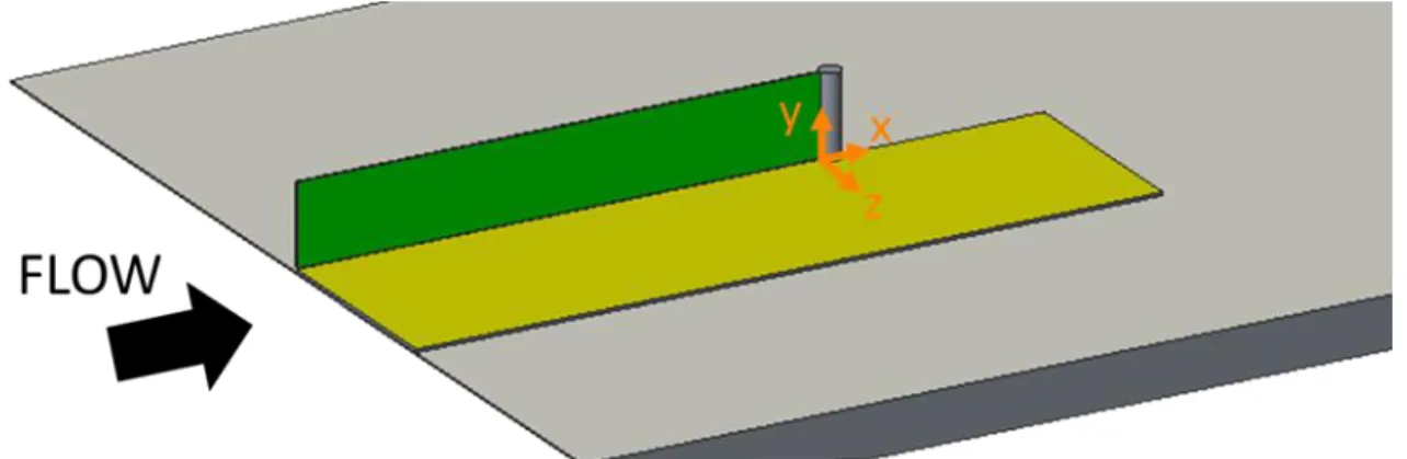
Experimental work in the past has primarily focused on the upstream region of a cylinder-induced interaction [14]. In particular, non-intrusive flow diagnostics, such as Schlieren and PIV, have typically been performed along the upstream centerline of the streamwise-transverse plane, as indicated by the green plane in Figure 2.1. Additionally, intrusive flow visualization techniques, such as oil flow visualization and pressure-sensitive paint (PSP), have typically been performed in the streamwise-spanwise plane, on the surface that generates the boundary layer, as shown by the golden plane in Figure 2.1.

(22)

In the x-y plane, for so-called “semi-infinite” cylinder- and blunt-fin-induced interactions, a lambda shock structure exists in the upstream region on the horizontal centerline, as indicated by the schematic in Figure 2.2. The diameter of the cylinder, d, is one of the dominant factors of the interaction scale, and all other parameters are thus normalized by d. The height of the cylinder, h, is also of particular importance because it dictates whether the interaction is considered semi-infinite or a function of h/d [11, 12] and

δ/d [12], where δ is the incoming boundary layer height. Dolling and Bogdonoff [12] identified this semi-infinite requirement as h/htp > 2-3, where htp denotes the triple point

height, and also estimated a guide of h/d > 2.4. Özcan and Yüceil [14] reported that this should be at h/d > 2.5, but used larger increments in their tests. Once the semi-infinite height is met, increasing h no longer changes the interaction structure. The interactions considered in this work are semi-infinite. In Figure 2.2, flow separation occurs at the separation length, λ, and generates an oblique shock, known as the forward shock, with

Figure 2.2. Front view schematic of a cylinder-induced shock wave/boundary layer interaction.

(23)

forward shock angle φ. This forward shock impinges upon the inviscid bow shock, which has stand-off distance B, at the triple point, where a bifurcation leads to the development of the trailing shock. Underneath the lambda shock, a separation bubble is formed, which consists of several vortices. The vortex structure varies depending on the state of the incoming boundary layer, and is discussed below for turbulent and laminar interactions. The trailing shock does not come into contact with the floor, but instead ends where it intersects with the separation bubble.

In the x-z plane, the separation shock is seen to curve outboard, as shown in Figure 2.3. Note that this view only refers to the floor surface and does not include the trailing shock, as this ends at the separation bubble. The largest extent of the separation shock is on the centerline with length λ, and as horseshoe vortices wash outboard, the distance between the cylinder and separation shock line is reduced. Vortex shedding also occurs just downstream of the cylinder, but this is symmetric in a statistical sense.

Figure 2.3. Top view schematic of a cylinder-induced shock wave/boundary layer interaction, indicating the surface interaction.

(24)

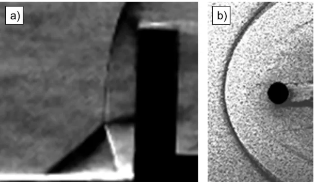
Sample Schlieren imaging and oil flow visualization from Lash et al. [6] for a turbulent interaction are shown in Figure 2.4a and b, respectively, and allow for a qualitative comparison to the schematics in Figure 2.2 and Figure 2.3, respectively. Note that all of the blue lines in the schematics are visible in the sample experimental results.

2.2 Turbulent Cylinder-Induced Interaction

As the turbulent interaction has the most practical applications, it is discussed first. The separation length is one of the key parameters of interest; Westkaemper [11] identified that

λ/d remains constant at approximately λ/d = 2.65 for an interaction where h/d > 1.13 over

M∞= 2.0-21, where M∞ represents the freestream Mach number. This was also observed

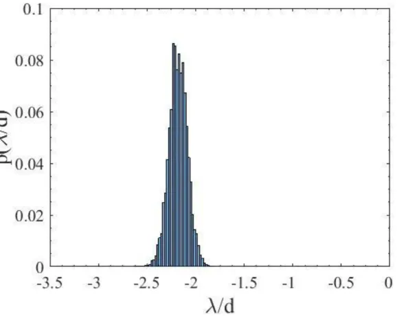
by Dolling and Bogdonoff [12] and Brusniak and Dolling [13]. However, experimental work by Lash et al. [6] and Combs et al. [7], and computational work by Yamamoto and Takasu [15], have all reported values closer to λ/d = 2.0-2.4. A distribution of separation lengths from the in-house work of Lash et al. [6] is shown in Figure 2.5, which indicated a

Figure 2.4. Sample a) Schlieren imaging and b) oil flow visualization for a turbulent interaction. Figure from Lash et al. [6].

(25)

Figure 2.5. In-house experimental results indicating probability density function of separation length. Figure from Lash et al. [6].

mean value of around λ/d = 2.15. These discrepancies may have arisen due to differences in Reynolds number, Re, or δ, which both affect the scale of the interaction [12, 13, 16]. The effect of δ/d at a constant Re will be investigated more closely in this study.

Westkaemper [11] also generated empirical equations for the remaining parameters of interest that are shown in Figure 2.2. The forward shock angle φ was determined by first finding the pressure coefficient, CP, through Equation (2-1) [17], where 5.61 is an empirical

constant, M∞ is the freestream Mach number, Rex is the local freestream Reynolds number

at location x, γ is the ratio of specific heats, and P is the static pressure, and then applying oblique shock relations via the pressure ratio [18]. This is used in conjunction with B, which is found via the empirical Equation (2-2) [11], in order to determine a geometric formula for h , which is shown in Equation (2-3) [11].

(26)

𝐶_𝑃 = 5.61 √𝑀∞𝑅𝑒𝑥 5 = 2 𝛾𝑀₁2( 𝑃2 𝑃₁ − 1) (2-1) 𝐵/𝑑 = 0.19 + 1.2 𝑀∞2 − 1+ 0.7 (𝑀∞2 − 1)2 (2-2) ℎ_𝑡𝑝/𝑑 = (𝜆/𝑑 − 𝐵/𝑑) tan (𝜑) (2-3)

The separation length is directly linked to a pressure rise in the upstream region. Pressure ratios comparing the computational data from Hung and Buning [16] with experimental data from Dolling and Bogdonoff [19] for a blunt fin interaction at M∞= 2.95,

shown in Figure 2.6a, indicated an initial pressure rise near x/d = −3. However, Hung and Buning [16] calculated separation to occur around λ/d = 1.7 in 1985, as indicated by the streamlines in Figure 2.6b, at a point where the pressure ratio had already risen near its initial plateau. This pressure plateau was followed by a trough that retained P/P∞ > 1, where

P∞ is the freestream pressure,which was then followed by the peak pressure just upstream

of the blunt body. Computational results, which are able to resolve this near-wall region at a much greater ease than experiments, predicted the peak pressure location around x/d = −0.1 [15, 16]. There was a pressure decrease just downstream of the peak pressure that reached yet another trough around x/d = −0.05, followed by a small pressure increase [15, 16]. This study will attempt to identify the reason for the peak pressure location, which would allow for mitigation of this critical parameter.

Streamlines, such as those shown in Figure 2.6b, provide a more in-depth understanding of the vortex structure and underlying flow physics, and will be used to characterize the flow. Note that there is a discrepancy between the steady-state computational result from Hung and Buning [16] and the time-accurate computational result from Yamamoto and Takasu [15]. The steady-state result [16] indicated a single, large, primary vortex, as shown in Figure 2.6b, but the time-accurate result [15] indicated a set of smaller, counter-rotating, primary vortices; this set varied between one and three vortices over time. The variation in the number of primary vortices was also observed by Sedney and Kitchens [20], and this variation for the steady-state result is likely attributed

(27)

Figure 2.6. a) Blunt fin pressure ratio comparing computational results from Hung and Buning [16] with experimental results from Dolling and Bogdonoff [19] at M∞ = 2.95, b)

Streamlines of the computational results on the upstream centerline. Figures from Hung and Buning [16].

(28)

to the differences in the modeling approach. However, there may also be a factor due to the unsteadiness in the interaction, such as the combined low- and high-frequency oscillations within the lambda shock structure. Lash et al. [6], Clemens and Narayanaswamy [10], Brusniak and Dolling [13], and Dolling and Brusniak [21] have all investigated this behavior and concluded that the forward shock undergoes low-frequency oscillations (f < 1 kHz), whereas the separation bubble, and hence the trailing shock, undergoes high-frequency oscillations (f ≥ 1 kHz). As the present study focuses on

steady-state interactions, a characterization of the frequencies will not be made; however, it is important to remember that the flow is inherently unsteady, and that this affects the vortical structure, among other things, for a steady-state result.

2.3 Laminar Cylinder-Induced Interaction

As laminar boundary layers are generally more susceptible to flow separation than turbulent boundary layers [22, 23], the scales of the interactions are inherently greater. While the initial pressure rise and flow separation for a turbulent interaction occur near x/d

= −3 and λ/d = 2.65, respectively, these values are approximately x/d = (−9)-(−6) for a laminar interaction [8]. Leidy et al. [24] found separation to occur closer to λ/d = 5.5-6 at

M∞ = 6. Itoh and Mizoguchi [25] and Mortazavi and Knight [26] note that similar unsteady

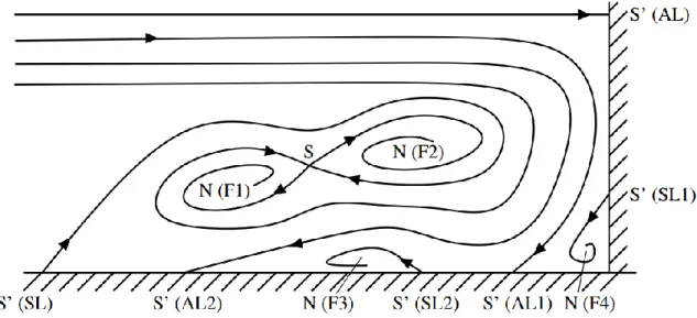
behavior exists for a laminar interaction as for a turbulent interaction, and have estimated Strouhal numbers from St = 0.032-0.113 through experiments [25] to St = 0.697 through computation [26], in contrast to St = 0.023-0.035 [27] for a turbulent interaction. A schematic of the vortex structures for a laminar interaction is shown in Figure 2.7, where

N, F, S, and S’ represent nodes, foci, saddles, and half-saddles, respectively. Furthermore,

AL represents an attachment line and SL represents a separation line.

Present computational capabilities lend themselves well towards solving laminar interactions. Knight and Degrez [5] and Holden [28] state that aerodynamic and thermal loads are accurately predicted using RANS simulations given that the mesh is adequately resolved. Holden [28] notes that gridding and numerical issues, in particular, have taken a long time to address and overcome, but have now fully matured. Dolling [4] states that grid-adaptation is an essential tool in solving laminar interactions.

(29)

Figure 2.7. Schematic of streamlines indicating vortex structure for a laminar interaction. Figure from Itoh and Mizoguchi [25].

The empirical equations for a laminar interaction are very similar to those for a turbulent interaction. Since the bow shock is inviscid, Equation (2-2) does not depend on the state of the incoming boundary layer, and thus remains valid. Furthermore, Equation (2-3) is a geometric formula and is thus also valid. The difference occurs in φ, which was calculated through CP in Equation (2-1). Truitt [17] proposed an alternate version, shown

in Equation (2-4), which was valid for a laminar boundary layer. Note that the constant of 17 differs from that of a turbulent interaction and was found through an iterative process until the pressure ratio matched a guessed value. The constant was not proposed by Truitt [17] and not verified under other flow conditions, and may not hold valid in a different interaction. 𝐶𝑃 = 17𝑀∞ √𝑅𝑒𝑥 = 2 𝛾𝑀₁2( 𝑃2 𝑃1 − 1) (2-4)

(30)

2.4 Transitional Cylinder-Induced Interaction Bounds

Addressing the scales of separation length and triple point height for the limiting cases of laminar and turbulent interactions paves the way for further research into transitional interactions. Kaufman et al. [8] have stated that the parameters of interest for a transitional interaction are confined to the values obtained by laminar and turbulent interactions. This is visible in Figure 2.8, which shows the separation length for each type of boundary layer using kerosene lampblack flow visualization at M∞ = 5, with flow from top to bottom.

Moreover, Kaufman et al. [8], Lash et al. [27], and Murphree et al. [29] have shown that a transitional interaction exhibits traits closer to those of a laminar interaction near the centerline, and closer to those of a turbulent interaction near the outboard extents.

Figure 2.8. Kerosene lampblack flow visualization from top view of shock wave/ a) laminar, b) transitional, c) turbulent boundary layer interactions at M∞ = 5. Flow from top

(31)

CHAPTER 3 METHODOLOGY

The simulations were run on two high-performance desktops that used the operating system Ubuntu 16.04 (64-bit) and contained 64 cores of the type AMD Opteron™ Processor 6376 at 2300 MHz each, along with 256 GB RAM. Furthermore, a cluster was available that ran the operating system Red Hat® Enterprise Linux® Server 7.2 and contained 11 nodes at 32 cores each (352 total) of the type Intel® Xeon® E5-2630 v3 at 2400 MHz each, along with 64 GB RAM per node. This computing power was sufficient for the simulations performed. Mesh generation was performed using Pointwise, Inc., V17.3R4, and post-processing was conducted using Tecplot, Inc., 360 EX 2015 R2.

3.1 Flow Modeling Assumptions

This study assumed a continuum model for the supersonic flow. As such, the fluid could be modeled using scalars for density, ρ, temperature, T, and the velocity components

u, v, and w. Air was the fluid of interest and was treated as a compressible, viscous, Newtonian fluid, and moreover as an ideal (or perfect) gas. The dynamic viscosity, μ, was determined via Sutherland’s law [30, 31]. Stagnation conditions were assumed to be constant; and since RANS provides a statistical mean flow, this flow was considered to be steady-state.

Further physical assumptions that were made in this study include the use of smooth, adiabatic, no-slip walls on the boundaries of the wind tunnel walls, flat plate surface and strut, and on the cylinder. The cylinder was initially modeled at the same height in the experiment, but this was ultimately increased to ensure a semi-infinite behavior for an analysis concerning the height of the incoming boundary layer, which directly affects htp

and thus h/htp. The flat plate leading edge, which was machined to be considered sharp,

was modeled with a blunt leading edge of radius 127 μm (0.005 in) [32], which was representative of the machining tolerance. Lastly, the wind tunnel was assumed to provide flow with a freestream turbulence intensity of 3% and a turbulent-to-laminar viscosity ratio of 5.

(32)

3.2 Numerical Formulation

3.2.1 Governing Equations

Reynolds-averaged Navier-Stokes simulations were performed using Metacomp Technologies, Inc., (Metacomp) CFD++ v16.1 [33]. The compressible, perfect gas Navier-Stokes equations were solved in dimensional, Cartesian coordinates, and are listed in Equation (3-1), where Q is the dependent variable vector, H is an inviscid flux vector, and

G is a viscous flux vector, as respectively described by Equations (3-2), (3-3), and (3-4). In Equation (3-1), Ṡ is the source term vector, and is zero except near physics source terms. The only source terms used in this study were at the far-field and are described later. Additional transport equations are solved when a turbulence model is active, and alter the terms μ and κ, the thermal conductivity, to be μ+μtand κ+κt, respectively. These transport

equations contribute to their own source term vectors. In Equation (3-3), E represents total energy. In Equation (3-4), 𝑞̇ represents the heat flux vector and τ represents the stress tensor. 𝜕𝑄 𝜕𝑡 + 𝜕(𝐻_𝑖+ 𝐺_𝑖) 𝜕𝑥𝑖 = 𝑆̇ (3-1) 𝑄 = [ 𝐸 𝜌 𝜌𝑢 𝜌𝑣 𝜌𝑤] (3-2) 𝐻𝑖 = [ (𝐸 + 𝑃)𝑢𝑖 𝜌𝑢𝑖 𝜌𝑢𝑢_𝑖 + 𝑃𝑛̂_𝑥 𝜌𝑣𝑢_𝑖 + 𝑃𝑛̂_𝑦 𝜌𝑤𝑢𝑖 + 𝑃𝑛̂𝑧] (3-3) 𝐺𝑖 = [ 𝑞̇_𝑖 − 𝑢_𝑗𝜏_𝑗𝑘 0 −𝜏_𝑖𝑥 −𝜏_𝑖𝑦 −𝜏_𝑖𝑧 ] (3-4)

(33)

3.2.2 Turbulence Model Set-Up

The turbulence models used in this study were Menter’s 2-equation shear-stress transport (SST) [34], the 1-equation Spalart-Allmaras (SA) [35] with quadratic constitutive relation (QCR) [36], simply referred to as SA-QCR here, and the 2-equation cubic k-ε

(CKE) [37]. All turbulence models were turned on at the 11th global time step, allowing for initial start-up transients to settle. The SST and CKE turbulence models used a turbulence under-relaxation parameter of 1, whereas the SA-QCR turbulence model used 0.75. The minimum level of turbulence quantities was 10−12 for all models, and the maximum ratio of turbulent-to-laminar viscosity was 1010 for all models. The Prandtl number was not directly specified, but maintained a laminar-to-turbulent Prandtl ratio of 0.8 and a turbulent Schmidt number of 0.7 for all models. Wall-functions were not implemented here. None of the turbulence models included baroclinic effects on production. The initial values for each turbulence model were computed with Metacomp’s turbulence initialization tool. [33]

3.2.2.1 SST

The SST model solves for the turbulence kinetic energy, k, and specific dissipation rate,

ω [38]. A wall-distance file was computed which was used to measure the distance from every cell to its closest wall [33]. Turbulence terms in the near-wall region were determined using Metacomp’s ε/ω boundary condition formulation v15.1 [33], but were also affected by the source terms, which depend on the wall-distance. Metacomp’s compressibility correction was implemented in combination with a wall-bounded flow type [33].

3.2.2.2 SA-QCR

The SA model solves for the kinematic eddy viscosity parameter, ν̃ [38]. Similar to the SST model, a wall-distance file was computed. The compressibility correction was implemented again for wall-bounded flows. The curvature correction was implemented to account for rotation and curvature effects [33], as these were strong factors in the interaction. These effects modified the calculation of ν̃ [33]. Also, the QRC option was enabled, which enhances stress predictions and improves performance in boundary layers. This option modified the Reynolds stress term [33].

(34)

3.2.2.3 CKE

The CKE model solves for k and turbulent dissipation, ε [38]. Metacomp’s compressibility correction for wall-bounded flows was active again. The dimensionless constant Cμ was formulated using the Goldberg formula [33], which is recommended for

flows with impinging or stagnating regions. The realizability criterion used Bradshaw’s constant [33], which is recommended for high-speed flow and for impinging or stagnating flow. The CKE model was not only used for the cylinder-interaction, but also to determine the flow conditions downstream of the flat plate leading edge shock and the growth of the boundary layer. As such, a leading-edge transition model [39] was implemented for this non-cylinder-interaction flow, which creates laminar flow near the leading edge until laminar separation is detected, after which the standard CKE model is applied [33].

3.2.3 Time Integration Set-Up

The steady-state solver was set to integrate the governing equations point-implicitly through the backward (or upwind) Euler method [38]. Simulations were run for 5000 global iterations to ensure that all residuals were flat-lined and no longer varied. The Courant-Friedrichs-Lewy (CFL) number was ramped linearly from 1 to 10 over the course of the first 100 iterations. When a divergence is detected in the solver, an automatic CFL number adjustment procedure (ACAP) takes place, which cuts the current CFL number in half and implements a new ramping schedule with a maximum of 0.95 times the CFL number when divergence was detected. A multi-grid W-cycle was implemented with 4 cycles and 20 levels. Non-strong agglomerations were allowed that were re-computed every 5 steps until the agglomeration had 1 group in its level. Time-step temporal smoothing was activated with a factor of 0.5. Time-step spatial smoothing was also turned on with 4 smoothing passes and a maximum time-step growth factor of 1.5.

3.2.4 Spatial Discretization Set-Up

The spatial discretization was 2nd_{order. A continuous total variation diminishing}

(TVD) flux limiter was applied with nodal base polynomial types and out-of-face viscous terms. A 1st_{to 2}nd_{order blending function for the backward Euler scheme was applied}

(35)

settled with a 1st order scheme before switching the solver to a 2nd order scheme. Typically, the residuals of the 1st order solution had dropped 4-5 orders of magnitude by the time the blend from 1st to 2nd order occurred.

3.2.5 Riemann Solver Set-Up

The Harten-Lax-van Leer-Contact (HLLC) scheme was used for the upwind discretization of the inviscid fluxes in CFD++ [33]. This approximate scheme, along with the TVD flux limiter, avoided oscillations [33]. A supersonic pressure switch was active which detected strong pressure gradients, i.e. shocks, and added dissipation in this region. Lastly, the carbuncle control was activated, which was used to reduce the dissipation error ahead of the bow shock in the nose region of the cylinder. This error arises when the solver switched from a hyperbolic to an elliptic method. The carbuncle control adjusted the maximum pressure factor to be 0.25.

3.3 UTSI Experiments

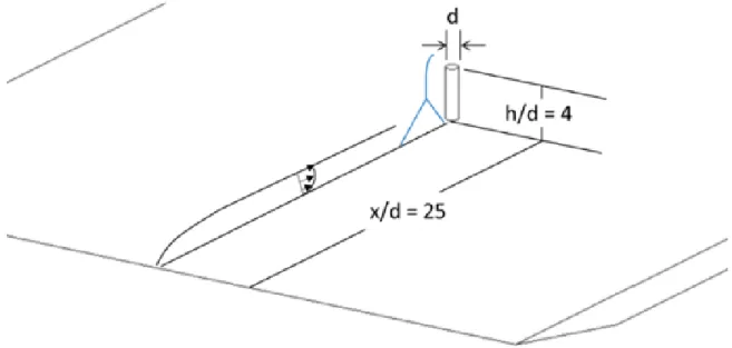
Experimental runs for a turbulent interaction were conducted by Lash et al. [6] and Combs et al. [7] at UTSI in a planar, low-enthalpy, blowdown wind tunnel with a test section size of 203.2 mm × 203.2 mm. High-speed Schlieren imaging [6] and 2-component PIV [7] were the two techniques employed for data collection. A 3.175 mm diameter, 12.7 mm tall brass cylinder was used to generate the interaction, resulting in an h/d = 4. The triple point was measured around htp/d = 1.4 [6], resulting in an h/htp= 2.85, which can be

considered semi-infinite according to Dolling and Bogdonoff [12]. The cylinder was mounted on a flat plate of 304.8 mm length × 203.2 mm width at a distance of 25d

downstream of the leading edge of the flat plate, as indicated by the schematic in Figure 3.1. This location has been verified to generate a fully turbulent interaction [6, 7].

The flat plate was angled downward at α = −2.9° in the experiment in an attempt to generate a zero pressure gradient on the upper surface. This angle was also applied to the CFD model by applying trigonometric identities to the u and v-velocity components. The coordinate system thus remained as initially indicated by Figure 2.2 and Figure 2.3. This configuration simplifies mesh generation and post-processing.

(36)

Figure 3.1. Schematic of the cylinder located on the flat plate.

The experiments have reported wind tunnel stagnation conditions, freestream velocity, and Mach number [6, 7], and have captured velocity and Mach number over the upper surface of the flat plate around x/d = −19.5 [7]. The wind tunnel stagnation conditions were used to calculate wind tunnel freestream conditions via isentropic relations [30], and oblique shock relations [18] were employed to determine the flow properties on the flat plate upper surface. The summary of these conditions, both reported and calculated, is provided in Table 3.1. As the coordinate system was angled, the wind tunnel freestream velocity of 507 m s−1 was decomposed such that u∞,WT = 506.8 m s−1 and v∞,WT = −25.67 m

s−1. This was not necessary for the flat plate upper surface, as the flow became tangential. The primary comparisons made between in-house experiments and the current numerical work were against the Schlieren work of Lash et al. [6], as the Schlieren data were more statistically robust than the PIV data from Combs et al. [7]. The parameters of interest, namely λ and htp, from Lash et al. [6] were directly used for comparison. Recall

from Figure 2.5 that a mean value of around λ/d = 2.15 was determined. Using B/d from Equation (2-2) along with the conditions in Table 3.1 and φ = 41°, obtained from Schlieren imaging [6], Equation (2-3) results in htp/d = 1.24, which was within 10% of the observed

(37)

Table 3.1. Flow conditions captured by experiments from Lash et al. [6] and Combs et al. [7] for wind tunnel and Combs et al. [7] for flat plate.

Wind Tunnel Conditions Flat Plate Conditions at

x/d = −19.5 P0 [kPa] 210.0 209.9 P∞ [kPa] 26.425 31.1 T0 [K] 286.8 286.8 T∞ [K] 158.6 166.2 Rem [m−1] 2.72 × 107 _{2.84 × 10}7 M∞ [-] 2.01 1.905 v⃗∞ [m s−1_] ₅₀₇ ₄₉₃

3.4 Domain Definition and Mesh Generation

Described below is the process with which the final computational domain was determined, and the specific details of that domain. The first simulation that was performed included not only the cylinder, but also the entire flat plate and strut, as well as the full width and height of the wind tunnel test section, as shown in Figure 3.2. A structured, hexahedral mesh was used with non-dimensional wall distance y+ = 30 and growth rate GR

= 1.2; therefore, wall functions were implemented to model the flow between the buffer layer and the surfaces. Note that this was the only simulation performed that used wall functions. The objective here was to determine whether or not the wind tunnel walls influenced the interaction, and the conclusion was that the walls were far enough away from the cylinder-interaction to allow for domain reductions.

Next, the problem was split up into 2 domains: one that solved for the flow over the flat plate upper surface, and one that solved for the cylinder-interaction, as based on a method employed by Chaudhry et al. [40]. The flow over the 2-D flat plate without the cylinder was solved first in order to accurately capture the boundary layer growth on the centerline. Then, slices of the flow perpendicular to the flat plate surface were taken and

(38)

Figure 3.2. 3-D domain of the first simulation using full width and height of the test section. This was used to test for sidewall influence and identify possible domain size reduction.

(39)

used as an inlet profile to the cylinder-interaction, whose domain was then represented by a 3-D box. The advantages to using this method were two-fold: first, the domain for the cylinder-interaction was smaller, therefore allowing for a finer mesh and thus better resolution; second, the domain for the cylinder-interaction was no longer bounded by the flat plate in the sense that various δ/d could be tested. Also, this method allows for the cylinder to be tested at various locations downstream of the leading edge of the flat plate without re-meshing, which may be beneficial in the future.

3.4.1 Flat Plate Flow

3.4.1.1 Initial Domain Size Reduction

As mentioned above, the full-test-section solution of the domain in Figure 3.2 indicated that a domain size reduction was possible, as there was no interference by the wind tunnel walls. Based on the freestream flow of the full-test-section solution, it was determined that the domain shown in Figure 3.3 would capture all of the flow physics, while also allowing for greater mesh refinement. The inlet boundary was extended to x/d = −30, or 5d (15.875 mm) upstream of the flat plate leading edge, in order to ensure there were no disturbances from the leading edge bow shock. The boundary condition applied to the inlet was a Musker

(40)

turbulent boundary layer profile [41], which used the wind tunnel freestream conditions from Table 3.1 along with a specified boundary layer height of 12.7 mm on the wind tunnel walls in order to develop a turbulent inlet profile that extended across the entire boundary. The streamwise extent was shortened to x/d = 15, and a zero-gradient outflow was applied as the downstream boundary condition. The domain extent beneath the flat plate lower surface was significantly reduced, as this minimally factored into the flow over the upper surface. Nevertheless, a small domain section at the lower surface was maintained to allow for the bow shock to develop on both sides of the flat plate, and thus rule out any blockage. As before, the outlet boundary condition at the lower surface was a zero-gradient outflow. A comparison with the full-test-section solution indicated that there was no change to the flow on the upper surface, and so this reduction at the lower surface was deemed feasible. The upper height of the domain was reduced to y/d = 20 at the inlet and approximately y/d

= 18 near the outlet. The far-field boundary conditions were set to a characteristics-based inflow/outflow, which is Metacomp’s far-field-type boundary condition.

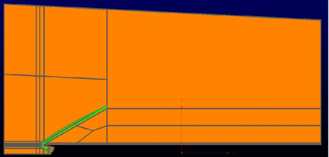
The final mesh for the domain of Figure 3.3 is shown in Figure 3.4. A first-pass was conducted with a structured, hexahedral mesh in order to more accurately determine the shock locations. Based on this, the final mesh was reconfigured for shock-alignment, as indicated by the green lines. A close-up of the flat plate leading edge, indicating the bow shock and two Mach waves emanating from the surface near the leading edge, is shown in Figure 3.5. This mesh consisted of hexahedral cells as well, but with the exception of a few unstructured, tetrahedral domains that can be identified in Figure 3.5 by the triangular domain zones. A total of 7 unstructured, tetrahedral domain zones (out of 83 total) were necessary to match the angled, shock-aligned domain zones with the surface. The walls were created with y+ = 1 and GR = 1.1, such that the entire mesh consisted of 1.2 million cells.

3.4.1.2 Final Domain Size Reduction

An attempt was made to further reduce the boundary height, since the freestream conditions downstream of the flat plate leading edge shock were relatively constant. Simply coarsening the mesh in this region was found to be inappropriate, as it under-resolved the

(41)

Figure 3.4. Medium 2-D flat plate mesh in x-y. Mesh domain zones are shown in grey, and shock-alignment is shown in green.

Figure 3.5. Close-up of leading edge section of the medium 2-D flat plate mesh. Mesh domain zones are shown in grey and shock-alignment is shown in green.

(42)

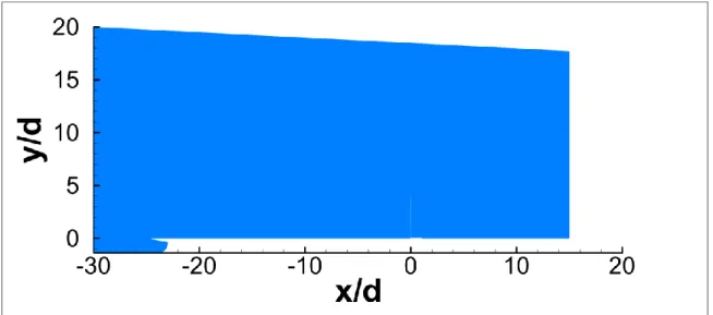
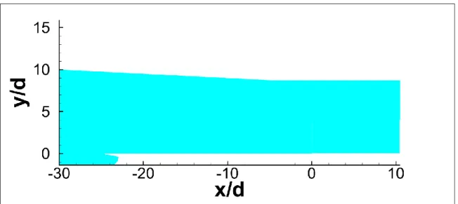
shocks and smeared them over several cells. Therefore, the height of the upper domain was reduced to y/d = 10 at the inlet and approximately y/d = 8.7 at the outlet, with the goal that the cell count could be reduced while increasing the accuracy of the solution. This height-shortened domain is shown in Figure 3.6.

Since the flow above the upper surface becomes tangential to the surface, the upper boundary above the flat plate may follow suit. From the flow solution for the domain of Figure 3.3 it was determined that despite the far-field condition being implemented, the flat plate leading edge shock had not dissipated out by the time it reached the upper boundary, and was reflecting back into the domain. This reflection impinged onto the flat plate boundary layer. In order to mitigate this issue, far-field absorbing layers were applied to the upper boundary. These posed the only contribution (other than the turbulence model) to the source term vector, Ṡ, in the RHS of Equation (3-1). Physically, the absorbing layers acted as a sponge boundary, where the flow was damped to user-specified freestream values over the course of several layers. The shock dissipated within these damping layers and did not reflect back into the domain, thus allowing for the implementation of the domain in Figure 3.6. The walls here were created with y+ = 0.1 and GR = 1.1; the fineness was required to properly resolve the small boundary layer in the vicinity of the leading

Figure 3.6. Smaller 2-D flat plate domain with reduced upper flat plate surface extent, and reduced height.

(43)

edge. A comparison between the solutions generated by the domains of Figure 3.3 and Figure 3.6 yielded no significant difference in the freestream or on the boundary layer.

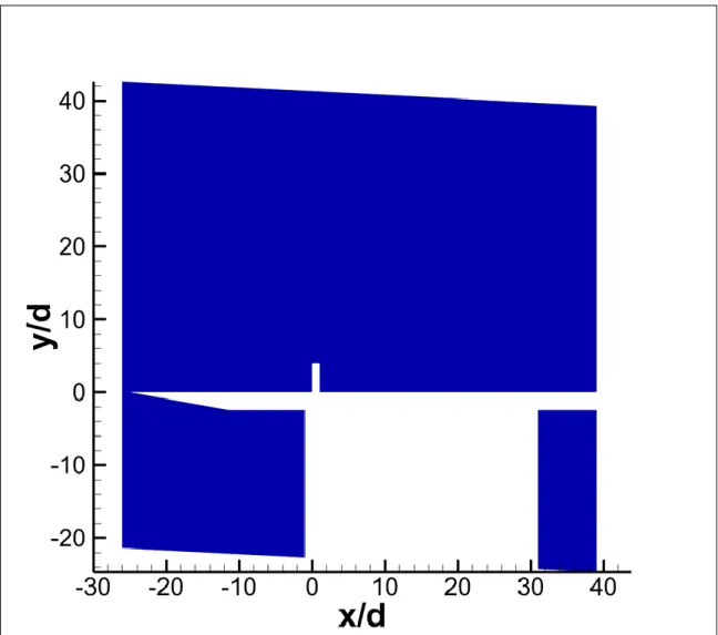
3.4.1.3 2-D and 3-D Comparison

In order to assess the extent of the turbulent cylinder-interaction, and to provide a comparison between the 2-D and 3-D flows over the flat plate, a 3-D version of the domain in Figure 3.6 was generated. The domain for this 3-D version is shown in Figure 3.7 and used the same dimensions as those in Figure 3.6. The mesh for the domain in Figure 3.7 was created in two directions: the flat plate flow remained in the x-y plane and the mesh from Figure 3.4 was extruded to z/d = 5. The cylinder-interaction section was created in a similar manner, where a base mesh in x-z was generated, as shown in Figure 3.8, and extruded first to match the height of the cylinder at y/d = 4. Then, the top of the cylinder was closed off and the mesh was extruded again to match the local domain height of approximately y/d = 8.7. The extrusion matched the cell spacing for each respective case. For the cylinder-interaction mesh in Figure 3.8, the same y+ = 1 and GR = 1.1 was applied. Furthermore, the radial section extended r/d = 3 outboard and had non-dimensional wall- distance of r+= 1 with GR = 1.2 in the radial direction, and constant azimuthal spacing Δθ = 30, as normalized by y+. The total extent for the cylinder-interaction base mesh was from

x/d = −5 to x/d = 10.5 and from z/d = 0 to z/d = 5, and the base domain contained a total of around 270 thousand cells. The full 3-D mesh with both the flat plate domain extruded along z and the cylinder-interaction domain extruded along y totaled approximately 19.8 million cells. At the interface between the two meshes, a zonal interface was generated to connect the cell faces with one another. This was implemented as a zonal boundary condition in CFD++. Additionally, the use of a symmetry plane is visible in Figure 3.8, which cut the cell count in half. The use of the symmetry plane was tested by only running the cylinder-interaction mesh both with and without symmetry, and it was verified that the symmetry plane was a valid assumption.

Simulations were performed with the CKE turbulence model. The reasons for this were two-fold: first, the CKE turbulence model contains a leading-edge transition model [33] that allows for a laminar section near the flat plate leading edge, thus providing a more

(44)

Figure 3.7. 3-D flat plate domain with cylinder, used to measure the extent of the interaction.

Figure 3.8. Base mesh of cylinder-interaction in x-z. Grey lines indicate domain zones, black lines show actual cells.

(45)

accurate representation of the boundary layer development; second, the Musker turbulent boundary layer profile requires turbulence inputs of k and ε [33, 41], and rather than converting turbulence values, it was convenient to directly implement these values from the CKE model solution. As for the initial conditions, a two-box method was implemented. The first box encompassed the entire domain space and used the primitive values from Table 3.1; the second box was formed in the wake of the cylinder and used the same primitive variables, except that u∞= 1 m s−1 in order to allow for the wake to develop by

itself. A comparison between the 2-D and 3-D flat plate solutions yielded no significant differences along the centerline. The extent of the cylinder-interaction was measured, and initial upstream disturbances occurred around x/d = −3. As such, the radial extent of the base mesh in Figure 3.8 was deemed reasonable, as it fully encompassed the pressure onset of the interaction. This will be shown in a later section.

3.4.1.4 Inlet Profiles

A final comparison was done between freestream results from the PIV experiment of Combs et al. [7] and the 3-D flat plate with cylinder CFD result at x/d = −19.5, as summarized in Table 3.2. There was excellent agreement among all primitive variables, as they were within 1% of the experiment. Due to this agreement, the slice profiles at x/d = −19.5 and x/d = −5 were used as inlet profiles for the laminar and turbulent interactions, respectively. Note that PIV data from Combs et al. [7] does not exist at x/d = −5, so a direct comparison could not be made. Also note that the boundary layer height was not captured by PIV data, but was estimated in collaboration with Schlieren images by Lash et al. [6] around δ = 0.32-0.48 mm (0.1d-0.15d). This is in good agreement with flat plate boundary layer theory by Schlichting [31]. As the numerical values fall within this range, the absolute value of the relative difference is assumed to be 0%. Since the PIV data considered the mean flow field, the CFD slices also averaged the freestream values from y/d = 1 to y/d = 2. Due to a non-zero pressure gradient being present on the flat plate, the primitive values still changed slightly, and this averaging was necessary; additionally, this explains the variation at the further downstream location of x/d = −5.

(46)

Table 3.2. Comparison between flat plate freestream conditions from CFD and PIV by Combs et al. [7] at x/d = −19.5, along with CFD data from x/d = −5.

x/d = −19.5 Experiment x/d = −19.5 CFD |Relative Difference| x/d = −5 CFD P∞ [kPa] 31.1 31.409 0.99% 31.837 T∞ [K] 166.2 167.2 0.60% 168.0 u∞ [m s−1] 493 490.2 0.57% 488.5 M∞ [-] 1.905 1.891 0.73% 1.880 δ [mm] (0.32-0.48) 0.407 (0.00%) 1.15 3.4.2 Turbulent Interaction

Similar to the flat plate domain, the domain for the turbulent interaction was also progressively reduced. The first iteration used the same domain as the base mesh shown in Figure 3.8, where a box was considered with extents x/d = −5 to x/d = 10.5, y/d = 0 to y/d

= 10, and z/d = 0 to z/d = 10. The second iteration decreased the height to y/d = 5 in order to reduce the cell count, and no significant differences were encountered in any of the parameters of interest. The third iteration decreased the height to y/d = 4, such that the upper boundary of the domain ended at the height of the cylinder. This method was also employed by Yamamoto and Takasu [15] and Hung and Buning [16], as it simplifies mesh generation. However, the scale of the interaction was decreased, as λ, and thus htp, were

both smaller for this iteration, and so this iteration was invalid. The fourth iteration decreased the downstream extent to x/d = 8; again, no significant differences were encountered in any of the parameters of interest. It was ensured that the entirety of the subsonic region generated by the wake of the cylinder remained upstream of this outlet, and was found to extend downstream to about x/d = 6. A large set of results was gathered with the fourth iteration, where x/d = −5 to x/d = 8, y/d = 0 to y/d = 5, and z/d = 0 to z/d = 5, and is presented in Chapter 4. As will be discussed later, the semi-infinite consideration for these results was questionable for large δ/d, which led to a fifth domain being generated, where a cylinder of height y/d = 10 was simulated, and the upper boundary extended to the

(47)

height of the cylinder. Both the fourth and fifth iterations used the base mesh, as shown in Figure 3.9, and extruded this to their respective boundary heights. Similar to the mesh shown in Figure 3.8, this mesh contained only structured, hexahedral cells. The actual cells are not shown here because a grid independence study altered these for each iteration. The values used to generate each mesh iteration in the grid independence study are presented in Table 3.3. The values of Δy and Δr were held constant once the boundary layer growth reached the intended maximum value of Δymax or Δrmax. This ensured that the grid did not

become too coarse away from the wall. Other boundary conditions for this domain were similar to those for the flat plate domain. A Musker turbulent boundary layer profile [41] was implemented at the inlet with the freestream conditions from Table 3.2, including δ = 1.15 mm (0.3622d). A zero-gradient outflow was present at the outlet. The far-field for both the fourth and fifth iterations was once again a characteristics-based inflow/outflow, using the same freestream conditions as in Table 3.2, but only the fourth iteration used the far-field absorbing layers. Initial conditions were similar to the 3-D flat plate flow, where the same near-zero velocity box was established in the cylinder wake. Note that the cell count is lower for the cylinder with height y/d = 10, despite containing a larger domain. This is because a y+ = 30 with GR = 1.2 was applied to the top of the cylinder with height

y/d = 4, and thus required a higher cell count.