Shapelet Transforms for Univariate and
Multivariate Time Series Classification
Aaron George Bostrom
A thesis submitted for the degree of Doctor of Philosophy
University of East Anglia School of Computing Sciences
May 2018
c
This copy of the thesis has been supplied on condition that anyone who consults it is understood to recognise that its copyright rests with the author and that use of any information derived there from must be in accordance with current UK Copyright Law. In addition, any quotation or
Abstract
Time Series Classification(TSC) is a growing field of machine learning research. One particular algorithm from the TSC literature is the Shapelet Transform (ST). Shapelets are phase independent subsequences that are extracted from time series to form discriminatory features. It has been shown that using the shapelets to transform the dataset into a new space can improve performance. One of the major problems with ST, is that the algorithm isO(n2m4), where
nis the number of time series andmis the length of the series. As a problem increases in size, or additional dimensions are added, the algorithm quickly becomes computationally infeasible.
The research question addressed is whether the shapelet transform be improved in terms of accuracy and speed. Making algorithmic improvements to shapelets will enable the development of multivariate shapelet algorithms that can attempt to solve much larger problems in realistic time frames.
In support of this thesis a new distance early abandon method is proposed. A class balancing algorithm is implemented, which uses a one vs. all multi class information gain that enables heuristics which were developed for two class problems. To support these improvements a large scale analysis of the best shapelet algorithms is conducted as part of a larger experimental evaluation. ST is proven to be one of the most accurate algorithms in TSC on the UCR-UEA datasets. Contract classification is proposed for shapelets, where a fixed runtime is set, and the number of shapelets is bounded. Four search algorithms are evaluated with fixed run times of one hour and one day, three of which are not significantly worse than a full enumeration. Finally, three multivariate shapelet algorithms are developed and compared to benchmark results and multivariate dynamic time warping.
Acknowledgements
First and foremost I would like to thank my supervisor, Dr. Anthony Bagnall, whose continued patience and support has proved invaluable throughout this process. I would like to thank my friends and colleagues at UEA and especially those in the time series classification group who have supported me.
I would also like to extend my thanks to Dr. Ji Zhou, and his team over at the Earlham Institute, he has supported my development as a researcher during my write up period, and I look forward to working with the group as I begin the next stage of my career.
Most importantly I would like to thank my beautiful fianc´e Amy Fellows, who has been the mental and physical support I have needed during my PhD, patiently putting up with the long nights, and strange working hours, and of course my cat Nacho for staying up with me.
Finally I would like to thank my good friends, to my teacher Paul Fretter, my friends George Beard, Adam Garner, Hilton Pashley, Sophie Farenden, James Large, James Macnamara, Leo Wilkins, Joshua Ball, Danny Reynolds and Pratik Gurung you have been a source of laughter and fun and have helped me immensely and I cannot thank you all enough.
List of Figures
2.1 sDist diagram taken from Time-Series Shapelets [114]. . . 25
2.2 Simple orderline with two classes . . . 27
2.3 Image taken from Logical Shapelets [79]. . . 29
2.4 Image taken from Fast Shapelets [83]. . . 34
2.5 Early Abandon of a time series (T) and a shapelet (S) being compared using thesDist function. In the illustration on the left, S an T are pairwise compared using Euclidean distance. In the diagram on the right, S and T are compared using Eu-clidean distance which has an early abandon point illustrated. The diagram is taken from [115] . . . 39
2.6 Fully calculated orderline with two classes. . . 42
2.7 Partially calculated orderline with two classes. The series that have not been calculated are placed in best case positions. . . 42
2.8 A simple diagram of a two dimensional time series comparison using Independent and Dependent dynamic time warping. The image on the (left) isDT WD and the image on the (right) is DT WI. Image taken from [99] . . . 49
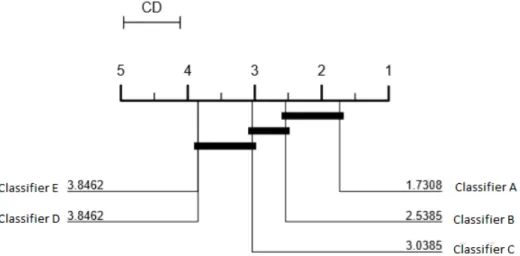
3.1 An example Critical Difference (CD) diagram demonstrating how to interpret the results from a pairwise comparison of five classifiers over multiple datasets. . . 53
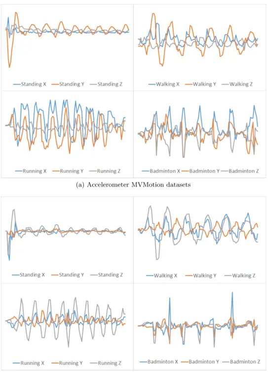
3.2 An example outline image created converted into a time series. 61 3.3 An example of the four classes for both Accelerometer data from the MVMotion dataset. . . 66
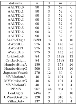
3.4 A list of the datasets in the multivariate time series archive. Number of instances is denoted by n, number of dimensions is denoted by d, length of series is denoted by m, and number of classes is denoted by c . . . 67
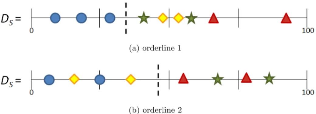
4.1 Critical difference of published results from Table 4.1 . . . 71 4.2 An example orderline split for two shapelets. Orderline (a)
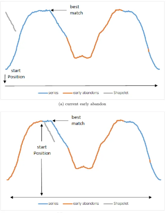
discriminates between class 1 and the rest, however orderline (b) has the higher information gain. . . 73 4.3 An example of Euclidean distance early abandon where the
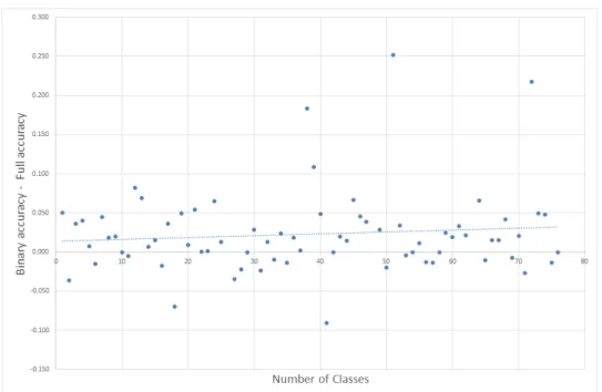
sDistscan starts from the beginning (a) and from the place of origin of the candidate shapelet (b). . . 77 4.4 Number of classes plotted against the difference in error
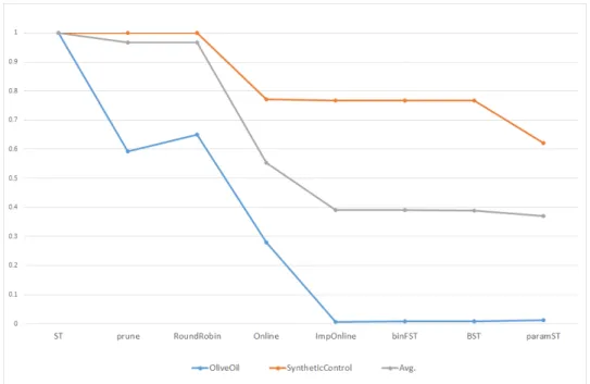
be-tween the full shapelets and the binary shapelets. A positive number indicates the binary shapelets are better. The dotted line is the least squares regression line. . . 80 4.5 The critical difference diagram of Table 4.3 . . . 84 4.6 The Average total opCounts performed for the 7 different
shapelets improvements. Average amount of work reduced,
shown with the best and worst dataset. (Oliveoil,SyntheticControl) 88 4.7 Normalised shapelet lengths with respect to series length for
all shapelets in the set used in the transformation process . . 89 4.8 Normalised shapelet lengths with respect to series length
for final shapelets for the datasets UWaveGestureLibraryX, UWaveGestureLibraryY and UWaveGestureLibraryZ . . . 91 4.9 The critical difference diagram of Table 1, (ST is an
abbrevia-tion for ST HESCA) . . . 96 4.10 The critical difference diagram of the best 9 algorithms from
5.1 All datasets able to fully enumerate the shapelet set in one day runtime. We demonstrate the calculated opcounts and timing estimate against the recorded data on the full transform with no optimisations, and the full transform with current state-of-the-art optimizations. . . 106 5.2 The proportion of accuracy relative to the full search. As the
sampling on the shapelet search areas increase the accuracy becomes worse and the variance increases. This demonstrates how random sampling breaks down in the extreme case. . . . 110 5.3 A heatmap demonstrating the quality of shapelets found in a
single series from ItalyPowerDemand . . . 113 5.4 A critical difference diagram comparing the four search
algo-rithms, with a runtime of one hour, and the Shapelet Trans-form via error. Three additional critical difference diagrams compare the four search algorithms by, balanced accuracy, f score and AUROC. . . 120 5.5 A set of four pairwise scatter plots demonstrating the accuracy
of the respective search algorithms with a runtime of one hour compared with the Shapelet Transform . . . 121 5.6 A critical difference diagram comparing the four search
algo-rithms, with a runtime of one day, and the Shapelet Transform via error. Three additional critical difference diagrams com-pare the four search algorithms by, balanced accuracy, f score and AUROC. . . 122 5.7 A set of four pairwise scatter plots demonstrating the accuracy
of the respective search algorithms with a runtime of one day compared with the Shapelet Transform . . . 123 5.8 A pair of critical difference diagrams presenting the preliminary
results of comparing 3 types of random subsampling with ST 124 5.9 A set of four box and whiskers plots showing the quality
of shapelets collected for each of the fourteen classes in the heartbeatBIDMC dataset. . . 126
6.1 Examples of Class 1 and Class 8 with their respective X, Y and Z multivariate series from the UWaveGesture dataset . . 129 6.2 Class Labels for the UWaveGesture dataset. Image taken from
[73]. . . 129 6.3 An example of extracting a single shapelet from a many
di-mensional series, and comparing it to a different series of the same dimension . . . 136 6.4 An example of extracting a ShapeletD from a many
dimen-sional series, and comparing it to a different series. Orange is the extracted shapelet, and blue is either the time series the shapelet is extracted from, or being compared too. . . 139 6.5 We present an illustrative example of extracting a ShapeletI
from a many dimensional series, and comparing it to a different series. Orange is the extracted shapelet, and blue is either the time series the shapelet is extracted from, or being compared too. . . 141 6.6 Accuracy and balanced accuracy of 10 algorithms using five
simple classifiers. These algorithms are RotationForest(RotF), RandomForest (RandF), Support Vector Machine using a quadratic kernel (SMO), Multi-Layer Perceptron (MLP) and 1 nearest neighbour with dynamic time warping (1NN DTW). We use the notation C to denote concatenation, and E to denote ensembled across dimensions. . . 142 6.7 Accuracy and Balanced Accuracy . . . 144 6.8 Two critical difference diagrams comparing the three shapelet
algorithms with the three multivariate dynamic time warping algorithms. . . 145 6.9 Four critical difference diagrams showing Accuracy, Balanced
Accuracy, AUROC and log likelihood of the best 12 algorithms. 149 6.10 Two critical difference diagrams showing accuracy and
bal-anced accuracy of the three multivariate DTW algorithms, the three timed shapelet algorithms and 1NN DTW on con-catenated data . . . 150
6.11 Four classes for the MVMotionA dataset . . . 151 6.12 Box and Whiskers plots of the quality of shapelets broken
List of Tables
2.1 Timing Results for ST, LS FS and STree in milliseconds. . . . 44
3.1 Number of datasets by problem type . . . 59
3.2 Electric Device Datasets . . . 60
3.3 ECG Datasets . . . 60
3.4 Image Datasets . . . 61
3.5 Motion Datasets . . . 62
3.6 Sensor Datasets . . . 63
3.8 Spectograph Datasets . . . 64
3.9 Distribution of Problem sizes . . . 64
3.7 Simulated Datasets . . . 64
4.1 Published Results for LS, FS and ST . . . 71
4.2 Number of data sets the binary shapelet beats the full shapelet split by number of classes. . . 81
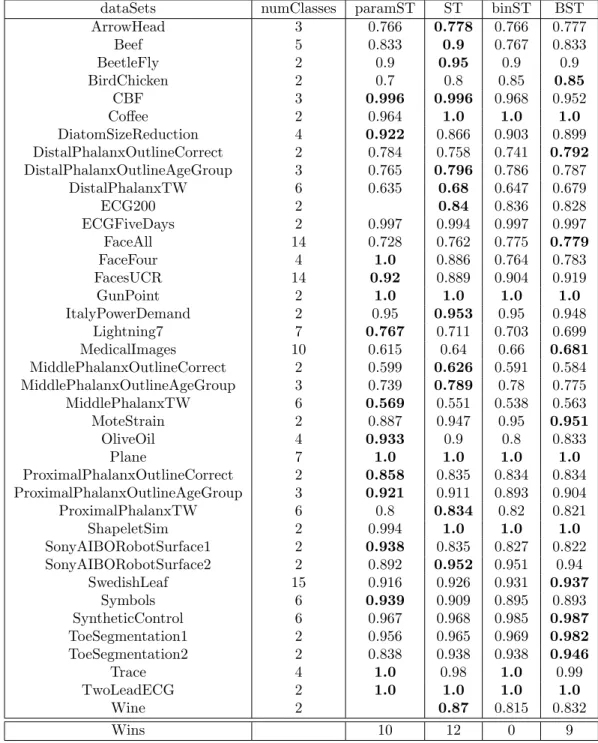
4.3 Table of the accuracies for the 4 variations of the shapelet algorithm, classified using HESCA . . . 83
4.4 A table of the seven different parameters used to measure the reduction in number of operations performed by the shapelet transform . . . 85
4.5 A Table showing the percentage of operations performed for each of the 7 parameter sets which are compared to a complete exhaustive search without optimisations. . . 87
4.6 Number of operations as fraction of the maximum amount of work, Averaged for all datasets . . . 88 4.7 Parameter Settings and ranges for Fast Shapelets and Learn
Shapelets. Consistent with original authors parameters . . . . 93 4.8 Two tables for the skipping parameters. (a) contains length
skipping, and (b) contains position skipping values . . . 94
5.1 One hour dataset list . . . 108 5.2 One day dataset list . . . 109 5.3 Table of average Accuracy conducted over 10 folds along with
the standard deviation . . . 125
6.1 A table of results for the Full searches for the three shapelet algorithms, and the three dynamic time warping algorithms . 146 6.2 A table of results showing the results for the one hour
run-times of the three shapelet algorithms using random shapelet selection and the three dynamic time warping algorithms. The standard deviation across the 30 folds is in brackets. . . 147
1 The average accuracies for the Shapelet Transform, Learn Shapelets and Fast Shapelets averaged over a 100 resamples for the 85 UCR datasets . . . 161 2 Two tables presenting a comparison of the overlapping fold 0
List of Algorithms
1 FindBestShapelet(T, min, max) . . . 27
2 checkCandidate(T, S) . . . 27
3 sDist(T, S) . . . 28
4 FindKBestShapelets(T,min, max, k) . . . 30
5 T ransf ormDataset(T,kShapelets) . . . 33
6 FindBestShapelet(Set of timeseriesT) . . . 35
7 FindBestShapelet(Set of timeseriesT) . . . 36
8 sDistCached(u, l, StatsA,B) . . . 41
9 BinaryShapeletSelection(T,min,max,k) . . . 74
10 sDist( shapeletS,seriesTi) . . . 78
11 FindKBestShapeletsWithSkipping(T,min, max, k, p, q) . . . 94
12 TabuSearch(T,Ti,min,max,ShapeletsT oEvaluate) . . . . 116
13 MagnifySearch(T,Ti,min,max,ShapeletsT oEvaluate) . . . 118
14 FindBestIndependentShapelets(MT, min, max) . . . 135
15 checkCandidate(MT, shapelet, d) . . . 135
16 sDistD(MT, M Shapelet, i, m, dimensions, l) . . . 138
Contents
List of Algorithms 1 List of Figures 1 List of Tables 6 1 Introduction 14 1.1 Introduction . . . 14 1.2 Motivation . . . 15 1.3 Contributions . . . 16 1.4 Thesis Organisation . . . 182 Technical Background and Related Work 20 2.1 Time Series Classification . . . 20
2.2 Time Series Classification Algorithms . . . 21
2.2.1 Whole series . . . 21 2.2.2 Intervals . . . 22 2.2.3 Shapelets . . . 22 2.2.4 Dictionary based . . . 22 2.2.5 Combinations . . . 23 2.2.6 Model based . . . 23 2.3 Shapelets . . . 23 2.4 Shapelet Tree . . . 24 2.4.1 Information Gain . . . 25
2.4.2 Shapelet Quality . . . 26
2.4.3 Brute Force Search . . . 27
2.5 Logical Shapelets . . . 28
2.6 Shapelet Transform . . . 29
2.6.1 Changes from Shapelet Tree to Shapelet Transform . . 30
2.6.2 Alternative Quality Measures . . . 30
2.6.3 Data Transformation . . . 32
2.7 Fast shapelets . . . 33
2.8 Learn Shapelets . . . 35
2.9 Fused Lasso Generalized eigenvector method . . . 36
2.10 Random Shapelet Tree and Random Shapelet Forest . . . 37
2.11 Efficiency Improvements . . . 38
2.11.1 Early Distance Abandon and Precomputing . . . 38
2.11.2 Entropy Pruning . . . 41
2.11.3 Similar shapelet abandon . . . 42
2.12 Shapelet Search improvements . . . 43
2.13 Timing Experiments . . . 43
2.14 Applications of Shapelets . . . 44
2.15 Issues With Current Approaches . . . 45
2.16 Multivariate Time Series Classification . . . 46
2.17 Multivariate Dynamic Time Warping . . . 48
2.18 Multivariate Shapelet Algorithms . . . 49
3 Experimental Methodology 51 3.1 Comparing Classifiers . . . 51
3.2 Performance Statistics . . . 54
3.3 Standard Classification Algorithms . . . 55
3.3.1 C4.5 Decision Tree . . . 56
3.3.2 Support Vector Machine . . . 56
3.3.3 Random Forest . . . 57
3.3.4 Rotation Forest . . . 58
3.4 Resampling Datasets . . . 58
3.6 Multivariate Datasets . . . 64
4 Improving the accuracy and reducing the runtime of the Shapelet Transform 68 4.1 Introduction . . . 69
4.2 Comparison of Published Results . . . 70
4.3 Multi-class information gain . . . 72
4.4 Changing the shapelet evaluation order . . . 75
4.5 Heterogeneous ensemble of standard classification algorithms 78 4.6 Results . . . 80
4.7 Analysing the individual Improvements . . . 81
4.8 Measuring heuristic speed up techniques . . . 84
4.9 Shapelet Distribution . . . 89
4.10 Resampling Experiments . . . 91
4.10.1 Results . . . 95
4.11 Conclusion . . . 97
5 Sampling the Shapelet Space 100 5.1 Introduction . . . 100
5.2 Quantifying the time for enumeration . . . 102
5.3 Sampling Shapelets . . . 109
5.4 Contract Sampling Algorithms for Shapelet Space . . . 111
5.4.1 Skipping search . . . 111
5.4.2 Random search . . . 112
5.4.3 Tabu search . . . 114
5.4.4 Magnify Search . . . 116
5.5 Experimental Comparison . . . 118
5.5.1 Subsampling Random Shapelet search . . . 123
5.6 Case Study: HeartbeatBIDMC . . . 124
5.7 Conclusion . . . 126
6 Multivariate Shapelet Transforms 128 6.1 Introduction . . . 128
6.3 Scaling the Shapelet Transform for Multivariate data . . . 132
6.4 Independent Shapelets . . . 133
6.5 Finding Multidimensional Shapelets . . . 136
6.5.1 Multidimensional Dependent Shapelets . . . 137
6.5.2 Multidimensional Independent Shapelets . . . 139
6.6 Evaluation . . . 141
6.6.1 Shapelets . . . 142
6.6.2 Comparing multivariate approaches with simple classi-fiers . . . 148
6.7 Case Study: MVMotionA . . . 150
6.8 Conclusion . . . 152
7 Conclusions and Future Work 155 7.1 Discussion of Contributions . . . 156
7.2 Future Work and Extensions . . . 158
Appendices 160
List of Publications
As First Author
• A. Bostrom and A. Bagnall. Binary shapelet transform for multiclass time series classification. Proc. 17th International Conference on Big Data Analytics and Knowledge Discovery (DAWAK), 2015
• A. Bostrom, A. Bagnall, and J. Lines. Evaluating improvements to the shapelet transform. Knowledge Discovery and Data Mining, in Workshop on Mining and Learning from Time Series, 2016
• A. Bostrom and A. Bagnall. Binary shapelet transform for multiclass time series classification. Transactions on Large-Scale Data and Knowl-edge Centered Systems XXXII: Special Issue on Big Data Analytics and Knowledge Discovery, pages 24–46, 2017
• A. Bostrom and A. Bagnall. A Shapelet Transform for Multivariate Time Series Classification. ArXiv e-prints, 2017
As Co-author
• A. Bagnall, J. Lines, J. Hills, and A. Bostrom. Time-series classification with COTE: The collective of transformation-based ensembles. IEEE Transactions on Knowledge and Data Engineering, 27:2522–2535, 2015
• A. Bagnall, J. Lines, A. Bostrom, J. Large, and E. Keogh. The great time series classification bake off: a review and experimental evaluation of recent algorithmic advance. Data Mining and Knowledge Discovery, pages 1–55, 2016
Chapter 1
Introduction
1.1
Introduction
Shapelets are subsequences of time series that are phase independent discrim-inatory features for Time Series Classification (TSC). TSC is a growing area of machine learning research. We consider time series data to be any ordered real-valued data. Time series classification is a specialization of the general classification problem. We define classification as: given a set of inputsx and outputsy, can we find a mapping from x to y? We define y as a set of unique labels where y ∈ {1, ..., C}. We assume that y = f(x) for some unknown functionf, and the goal of classification is to learn f from a set of labelled inputs so that ˆy = ˆf(x). Informally the goal is to learn from the labelled training data so that we can predict class membership of unknown series.
Classification relies on finding or deriving explanatory features, either through a probabilistic approach, or by measuring similarity to form group-ings and define decision boundaries. In traditional classification, and in simpler models, such as na¨ıve bayes, attributes are often treated as inde-pendent of one another. However, in TSC problems the ordering of the attributes can be critical in deriving explanatory features, and in being able to discriminate between classes. There has been a large amount of research
into algorithms for time series classification, some of which we review in chapter 2. Recently a large scale experimental evaluation [8] compared the best algorithms from the literature and found that transformation based approaches performed better on average. One of the best algorithms in this study was the shapelet transform [70].
1.2
Motivation
The shapelet transform (ST) was proposed in [70] where it was adapted from the the shapelet tree algorithm [114]. Shapelets are phase independent subsequences that are found within the time series data and they are covered in great detail in chapter 2. ST was shown to be a significant improvement over the tree based implementation, as the model was uncoupled from a decision tree and a better classification algorithm was paired with this shapelet transformed data.
One of the major problems with the shapelet tree algorithm, and sub-sequently the shapelet transform algorithm, was the run time. Shapelets were originally created because they capture phase independent features. These features could also be mapped back to the original series to derive data driven rules that could be interpreted by a human. The problem with this approach is that to find the global best features, a full enumeration of all subsequences in the datasets is required, which is very time consuming. There are three major motivations for this thesis. Firstly, to improve the classification accuracy of the shapelet transform by extracting better quality shapelets. In [72] different quality measures were evaluated for extracting shapelets. These methods can be problematic on multi-class problems when the number of classes is very high. The distribution of shapelets that can be found is largely dependent on the underlying class distribution of the training data. Where there is an imbalance in the distribution of classes in a dataset, this can adversely affect the number of shapelets found, as such we may need to compensate for this an evenly distribute the number of shapelets on a per class basis.
of the shapelet transform. The current runtime complexity of the shapelet transform isO(n2m4) wheren is the number of time series andm is their length. In chapter 2 we cover the early abandon techniques already proposed in the literature, the objective is to improve upon existing techniques. In other areas of Computer Science research time constrained algorithms exist for approximating difficult to solve problems. Shapelet finding could be an ideal candidate for heuristic search algorithms and time constrained learning.
The third motivation is to adapt ST for multivariate time series classi-fication. Multivariate time series data is becoming widespread, where the number of sensors and devices are able to capture vast quantities of data. One particular area of multivariate time series classification research is elec-troencephalography (EEG). Critically, very little shapelet based research has been conducted on multivariate data. Shapelets as a technique are only defined in the univariate case, the motivation is to define shapelets for the multivariate case, and leverage off the previous improvements to efficiency to enable multivariate TSC. The time complexity problem is only exacerbated as more data points are added. No free lunch theorem is present in many fields, and time series classification is no exception [111]. No single algorithm will generalise well to all problems and tailor made algorithms for multi-variate time series classification are required. However, we are motivated to assess current simpler approaches to see where they can compete with more hand-crafted solutions and provide benchmark results with which to compare.
1.3
Contributions
To provide support for this thesis, large scale experimentation were conducted and novel algorithms are proposed. The contributions of this thesis are as follows:
• Binary shapelet transform for multi-class time series classifi-cation. We present our novel algorithm for balancing binary shapelets, which leverages existing speed up techniques on multi-class problems.
A revised evaluation order is shown to reduce the number of funda-mental operations required in the average case compared to existing speed up techniques. A study of the multi-class datasets found in the UCR-UEA archive [23] found that the balanced shapelets improve the shapelet transform on multi-class problems. We present the concept of a shapelet transform that uses balancing and binary shapelets when the number of classes is greater than two, or otherwise reverts to the original. This work is reported in chapter 4 and published in [15, 16].
• The great time series classification bake off. This was a large experimental evaluation undertaken by the research group at UEA. An endeavour to implement the 20 most common algorithms from the TSC literature under a common framework and evaluate them on 8500 datasets. The contribution presented in this thesis in chapter 4 and used extensively in further comparisons in chapter 5 was implementing and testing the Learn Shapelets and Fast Shapelets algorithm on 8500 problems [83, 40] and comparing them with the Shapelet Transform presented in the first portion of chapter 4. These results were published in [8] where the Shapelet Transform was only beaten by COTE, of which the shapelet transform is a constituent. The Shapelet results contributed to the building of the COTE ensemble and the changes made to ST contributed in part to the improvements seen from the previous iteration which was presented in [6].
• Evaluating the shapelet transform. A converted Fast Shapelet algorithm is presented as a transform instead of a decision tree, and shown that it is significantly better than the tree implementation. However, the Fast Shapelet Transform is significantly worse than the Shapelet Transform, although it is considerably faster. We then present a contract shapelet algorithm where the stride parameters can be derived from a given time limit. These stride parameters enable the shapelet search to avoid areas of the search space and constrain it to a fixed runtime. It is shown that heuristically evaluating the search space is not significantly worse than a full enumeration and the work published
in [18] is improved upon by considering more complex heuristic search techniques in chapter 5.
• Shapelet Transform for Multivariate Time Series Classifica-tion. Three novel approaches to multivariate time series classification are described. These multidimensional shapelet algorithms are bench-marked against a number of common machine learning algorithms on multivariate datasets. Univariate classification algorithms are adapted to the multivariate data by either concatenating the dimensions into a single series or by forming a homogeneous ensemble on each dimen-sion. We have sourced and processed 24 datasets from the literature and converted them into a common format for use with the WEKA framework, building a foundation for the MTSC community to expand upon. The work and results are publicly available and are published in e-print [17], whilst also being under review.
1.4
Thesis Organisation
The remainder of this thesis is organised as follows. In chapter 2 a review of the time series classification literature, with a large emphasis on shapelet research is presented. In chapter 3 we describe the datasets we use to benchmark with, the way in which we conduct large scale experiments and some of the statistics we use to present and analyse our results. In chapter 4 we outline our first contribution, which aims to reduce the runtime of the shapelet transform and increase the classification accuracy on multi-class problems. In the second portion of chapter 4 we discuss our contribution to the work [8] and how these form the core of experimental methodology for later contributions, as well as the benchmark which we aim to maintain in chapter 5. The aims of chapter 5 are to build on the success of previous work and apply heuristic techniques from both the literature and a novel approach to finding shapelets in a fixed time frame. The final contribution is presented in chapter 6 where the speed up techniques developed in previous work are used in conjunction with the three novel shapelet approaches to
multivariate time series classification. This thesis is concluded in chapter 7 where the contributions are discussed and future work is considered.
Chapter 2
Technical Background and
Related Work
This chapter introduces some of the technical background used in this thesis. We introduce the problem of time series classification (TSC) and present a review of shapelet based techniques. The aims of this project are to improve Shapelet based classification as it was identified as one of the best time series classification algorithms from within the literature.
In this chapter we present a review of the history of the algorithm, and the various changes and optimisations published since its creation.
2.1
Time Series Classification
There are many types of problems that exist in time series data mining including clustering, classification, querying, forecasting and indexing. In this thesis the sole aim is to focus on shapelet based techniques for time series classification, where the class label is a constant singular value per series.
We define a set ofn time series as
where each series consist of mreal-valued attributes
Ti =< t1, t2, ..., tm >
and a class valueci.
Many TSC algorithms are based on measuring similarity between series. There are three major types of similarity in time series classification. These are similarity in time, similarity in shape, and similarity in change. Similarity in time is predominantly found using nearest-neighbour techniques with either Euclidean Distance (ED), or Dynamic Time Warping (DTW) [75, 51, 101, 85, 59, 60, 21]. Similarity in change is where the features of a dataset are embedded in the autocorrelation structure of the time series. An example is an Autoregressive Moving Average Model (ARMA) [25, 3]. Finally, there is similarity in shape. This is the major focus of this thesis. If the shape is local and embedded in the time series, subsequence techniques are needed [40, 114, 70, 83, 79].
2.2
Time Series Classification Algorithms
Bagnall et al. [8] conduct a thorough analysis of a large portion of the algorithms presented in the literature. The major algorithms are broadly separated into six simple groupings. The techniques are grouped into the following categories:
2.2.1 Whole series
Whole series algorithms tend to be based around adaptations and extensions of either the Euclidean distance (ED) or Dynamic Time Warping (DTW) [86]. These algorithms are paired with a nearest neighbour classifier and have seen relative success in large scale experimental comparisons [8]. Many variations of dynamic time warping exist and are covered thoroughly in [8]. Weighted Dynamic Time Warping (WDTW) was presented in [51] where they add a penalty to the warping distance. Time Warp Edit (TWE) was proposed to give a stiffness parameter to the warping [75]. Move-Split-Merge (MSM) is a
metric that is similar to other edit distance algorithms [101]. Other metrics include Edit distance with Real Penalty (ERP) [22] and Longest Common SubSequence (LCSS) [48]. Wang et al. [107] found that over 38 datasets 8 of these measures were not significantly better than DTW.
2.2.2 Intervals
Interval algorithms are described as finding phase dependent features. One of the main interval based approaches is Time Series Forest (TSF) [30]. The main problem with the phase dependent models is that the feature space is very large, they overcame this by using a random forest type approach. Each tree is generated with√mrandom intervals. These intervals are used to generated summary statistics which are used to build the tree, and classification is majority voting within the ensemble. Time Series Bag of Features (TSBF) [12] and Learned Pattern Similarity (LPS) [11] were proposed as extensions to TSF by the same group at Arizona University. On the UCR archive these methods were found to be not significantly better than each other.
2.2.3 Shapelets
These algorithms find phase independent subsequeneces from within the time series. Essentially these algorithms select subsets of contiguous features and build standard classification models on the features. Shapelets are the main focus of this thesis and the remaining sections in this chapter are dedicated to a large scale review of the shapelet based literature.
2.2.4 Dictionary based
Dictionary based classifiers are broadly based around the Bag Of Patterns model (BOP) which was proposed by [68]. BOP is a dictionary based classifier built on SAX [67]. SAX is covered in greater detail in section 2.7. The distribution of the SAX words in a series produce a histogram of the counts. The same data transformation is applied to new series, and a nearest neighbour of the histograms is used to classify. Symbolic Aggregate
approXimation-Vector Space Model (SAXVSM) combines SAX and a vector space model that is common in Information Retrieval. SAXVSM forms frequencies over classes rather than series, and uses Term-Frequency Inverse Document Frequency (TFIDF) to weight these histograms [95]. Bag of SFA symbols (BOSS) is different to BOP and SAXVSM in that is uses a Discrete Fourier Transform (DFT) instead of a Piecewise Aggregate Approximation (PAA) on each window [93] . The series are truncated using Multiple Coefficient Binning (MCB) rather than the fixed interval approaches of the previous sections. From the literature on the published 19 UCR datasets used, BOP and SAXVSM were not significantly better than each other, and both are significantly worse than BOSS.
2.2.5 Combinations
These algorithms combine one or more of the above approaches into a single classifier.
2.2.6 Model based
These types of algorithms are not well represented in the literature but they include auto-regressive models [9, 25], hidden Markov models [100] and kernel models [24]. These algorithms tend not to be used in classification [74].
2.3
Shapelets
Shapelets are a subsequence of a time series designed for finding local phase independent similarity. They were first proposed in [114] and have been a prominent area of TSC research since. We define a subseries of a time series of lengthl as a contiguous set of values from within a seriesTi. Any
contiguous series in a time series can be a shapelet, and so the maximum number of distinct shapelets in a single series is (m−l+ 1).
2.4
Shapelet Tree
The shapelet tree algorithm was one of the first algorithms in TSC aimed at finding similarity in shape [114, 115]. The brute force algorithm for finding shapelet and evaluating shapelets is presented in algorithm 1. The algorithm searches through the entire set of subseries within a dataset, evaluating the quality of each subseries, recording the best. The best subseries is selected as the shapelet which is then used as splitting rule in the decision tree, and the process continues on each sub-tree. The data is subdivided by the shapelet at each node until either a maximum depth is reached, or a sub-tree dataset contains all of one class.
Quality and Distance Measures
Information Gain is used to measure the quality of a single shapelet [97]. To calculate information gain a measure of similarity between shapelets and between a shapelet and a series is required. Euclidean distance is used to measure the similarity of two equal length series. Euclidean distance is defined in Equation 2.1, where A and B are series and they are of length l.
dist(A, B) = v u u t l X i=1 (Ai−Bi)2 (2.1)
In order to measure the distance between two series that are different lengths we need to define a separate function. sDist(S, T) is a function that uses a sliding window on the longer series, in this caseT, where the width of the sliding window is set to that of the shorter series. Each subseries inT
is compared to the input subseriesS. As these subsequences are the same length, they are compared using the Euclidean distance. This generates a set of distancesW which containsm−l+ 1 distance values. sDistfinds the best matching location in the longer series, and thus the smallest distance is considered the best. To illustrate this point, if S is extracted from T,
sDist(S, T) =minw∈W(dist(s, w))
Figure 2.1: sDist diagram taken from Time-Series Shapelets [114].
2.4.1 Information Gain
To evaluate the quality of a single shapelet, information gain [97] is used as a measure of how well it can separate two classes. Initially we present the formula for calculating information gain, and entropy, we then apply this to shapelets with a worked example.
Given a dataset D, with two classesC1 andC2, the proportion of time series which belong to classC1 is p(C1) and the proportion which belong to
C2 isp(C2), we define the entropy ofDas:
E(D) =−p(C1)log(p(C1))−p(C2)log(p(C2))
To determine the information gain we need to calculate the best split in the dataset D, we create two subsets D1 and D2 by splitting Dand then calculating the entropy ofD1 andD2 respectively. The entropy is calculated in proportion to the whole, so calculating the fraction of classes in D1 as
f(D1) and the fraction of classes in D2 as f(D2), the entropy of the split is: ˆ
E(D) =f(D1)H(D1) +f(D2)H(D2)
Given the definition of Entropy and how entropy of a given split is calculated. Information gain can be defined as the difference in the entropy
of the original set compared to the entropy of the two subsets.
I =E(D)−Eˆ(D)
2.4.2 Shapelet Quality
The quality of a shapelet is determined by using the distance from the shapelet candidate to every series in the dataset. This generates a list of
n distance values, which is called an orderline. An orderline consists of a pair of values, the distance value, and the class label for the respective series, and is sorted in ascending order based on the distance value. An ideal shapelet should produce small distance values when compared to time series of the same class and large distance values with other classes. The optimal configuration for an orderline is where all of the distance and value pairs in the orderline that are the same as shapelets class are located inD1 and all other pairs are located inD2.
A given orderlineO should contain ndistance and class value pairs. The orderline is sorted by the distance into ascending order. The number of splitting points that will generate unique information gain values isn−1. The shapelet algorithm calculates the information gain for all split points, selecting the maximum information gain, and corresponding split point. For clarity, a worked example is described. An orderline of 6distances with4 of class B and 2of class R is illustrated in Figure 2.2. The optimal split point is shown with a dashed line. The orderline splits the 6 distances into two sets. There are 3 total distances on the left and there are3 total distances on the right. The left hand side contains the elements inD1 of the equation. This side is simpler as there is only class B present which means there is only 3 of class B. The right hand side contains the elements in D2 of the equation, there are both classes B and R, where there are2of class R, and1 of class B. In Equation 2.2 the maximum informatio gain of the orderline from Figure 2.2 is calculated. The first section of the equation calculates the portion each class contributes towards the total set. This could also be described as the ideal entropy.
I = [−(4/6)log(4/6)−(2/6)log(2/6)] −(3/6)[−(3/3)log(3/3)] +(3/6)[−(2/3)log(2/3)−(1/3)log(1/3)]
(2.2)
Figure 2.2: Simple orderline with two classes
2.4.3 Brute Force Search
Algorithm 1 FindBestShapelet(T, min, max) WhereT is a set of Time Series.
best quality, quality best shapelet, shapelet
for Ti inT do
for l=mintomax do forp= 0 to|Ti| −l+ 1do
shapelet=Ti,pl
quality=checkCandidate(T,shapelet) if quality > best quality then
best quality=quality best shapelet=shapelet
return best Shapelet
Algorithm 2 checkCandidate(T, S)
WhereT is a set of time series andS is a shapelet candidate. WhereO is an orderline.
forTi inT do
dist=sDist(S, Ti)
O∪< dist, ci >
Algorithm 3 sDist(T, S)
WhereT is a time series andS is a shapelet candidate.
l=|S|
min dist=∞
forp= 0 to|T| −l+ 1do
dist=dist(S, Tpl) if dist < min distthen
min dist=dist
return min dist
The brute force search defined in algorithm 1 is slightly modified in contrast to the version in the the original paper [115]. This is to make it more in line with the implementation. The original algorithm description precomputed and stored all the possible shapelet candidates in a set. Instead the algorithm finds and evaluates each shapelet individually.
2.5
Logical Shapelets
Logical shapelets were an adaptation to the shapelet tree algorithm, Mueen et al. [79] proposed a statistics caching optimisation which is discussed in greater detail in subsection 2.11.1. The aim of logical shapelets is to combine shapelets to form more complex rules to better handle difficult to separate problems. The algorithm is a combination of shapelets used in conjunction with each other for determining the class separation on the orderline. In Figure 2.3 we illustrate one of the motivating examples which was presented in the original paper. In the diagram the first class (yellow) has two independent shapes that represent the class, but only where they appear together. The problem with distinguishing this from the other class is that the shapelets occurrence is independent from one another, therefore they cannot be represented as single shapelet and individually they cannot separate either class, thus producing a poor information gain value. The splits that are detected are then divided into either broken or non-linearly separable shapelets. These broken shapelets are evaluated with the logical shapelets, where additional shapelets are searched for to try and achieve a
better splitting.
Figure 2.3: Image taken from Logical Shapelets [79].
2.6
Shapelet Transform
The shapelet transform was proposed in [70] and further expanded upon in [47, 72]. A number of significant changes to the original algorithm were proposed, these included: separating the shapelet finding process from the classification model, considering alternative similarity measures and further speed up techniques to the sDist function. As was discussed earlier, the original shapelet algorithm was embedded in a decision tree, finding the best shapelet at each node recursively subdividing the data. This results in the brute force search being performed a number of times at each node, which makes it intractable on large problems. The shapelet transform algorithm does not change the brute force, but requires it is done only once. Separating the shapelet finding algorithm from classification meant that a number of the drawbacks of decision trees could be avoided. Decision trees are often out performed by other classifiers and they have a tendency to over fit unless post-pruned. The shapelet transform performs a data transformation by finding a set of k shapelets and creating a new dataset of k features per series. In algorithm 4 the single pass shapelet search for thek best shapelets
is proposed.
Algorithm 4 FindKBestShapelets(T,min, max, k) WhereT is a set of Time Series.
KShapelets=∅ forTi inT do
seriesShapelets=∅ for l=mintomax do
forp= 0 to|Ti| −l+ 1do
quality=checkCandidate(T,Ti,pl )
seriesShapelets=seriesShapelets∪ {Tli,p,quality}
sort(seriesShapelets)
removeSelf Similar(seriesShapelets)
kShapelets=merge(k, kShapelets, seriesShapelets)
2.6.1 Changes from Shapelet Tree to Shapelet Transform
Algorithm 4 describes the shapelet transform. This section describes the changes from the shapelet tree algorithm in more detail. The brute force search algorithm is the same as the one presented in algorithm 1. The tuning parameter k is the size of the final shapelet set, the other change is the forming of the shapelet set. As we consider each shapelet we create a list, which after each series has been considered, is sorted, and the self similar shapelets are pruned, and merged into the k best shapelets list. This process happens for each series. Self similar shapelets are formally defined in [47]. Informally, self similar shapelets are overlapping subsequences of varying lengths and starting positions. This ensures the best quality and longer non-overlapping shapelets are only considered when merging into the kShapelets set.
2.6.2 Alternative Quality Measures
Lines and Bagnall [72] proposed a number of alternative measures for assessing the quality of shapelets [72]. One of the problems with information gain is that the entropy pruning speed up, presented earlier in subsection 2.11.1, is not efficient on multi-class problems. Calculating the best possible configurations
of a two class problem is possible in constant time because the orderline is 2 dimensional. To find the best possible configuration of multiple classes becomes untenable and does not improve speed. Three alternative distance measures were proposed in [72], these were Kruskal-Wallis, F-statistic(F-stat) and Mood’s median [78, 62].
Given a set of n samples F-stat is used to analyse the variance in the difference of means. The statistic is used in Shapelets to test the variability of the distance between Shapelets and series, where low variability of series in the same class, and high variability between classes yields a good shapelet. The set of distancesO, our orderline is still required, thus the F-stat is not a complexity improvement, but it has been shown to be more effective than IG. Given our orderline of distances, we sort the distances and their class membership into separate sets,Oi, we also calculate the average distance in
Oi as ¯Oi and the average distance to all series as ¯O. We denote the number
of classes asC andn is the number of series. We calculate the F-stat value by: F = P i ( ¯Oi−O¯)2/(C−1) C P i=1 P dj∈Oi (dj −O¯i)2/(n−C)
Kruskal-Wallis is a non-parametric test which determines whether two groups are from a distribution with the same median [62]. Given our orderline of distance we sort the distances and their class membership into separate sets, Oi we also need a corresponding set of ranks, R, where the set of
distances inOi also correspond to Ri. We denote the average rank as ¯R and
the average rank of theith class as ¯Ri.
K = 12 n(n+ 1) C X i=1 |Ri|( ¯Ri−R¯)2
The final alternative quality measure proposed by [72] is Mood’s median. Similar to Kruskal-Wallis, Mood’s median is a non parametric test which wants to determine whether two groups are from a distribution with the same
median. Unlike Kruskal-Wallis and the other alternative quality measures, Mood’s median does not require the Orderline to be sorted. The measure first starts by creating a contingency table where the counts of each class above or below the median are recorded. It was shown that the median can be found inO(n) time [49]. Where ois the observations, and e is the expected. M = C X i=1 2 X j=2 (oij−eij)2 eij 2.6.3 Data Transformation
The major change from the Shapelet Tree algorithm to the shapelet Transform was the data transformation process. The data transformation is formally defined in algorithm 5. Given a set of a time seriesTand a set ofkshapelets kShapeletsthe algorithm calculates the minimum distance between each series and each shapelet. Anxk matrix is constructed from these distance values, in addition to the class values which are appended to the end of the series. The main aim of creating a transformation was to separate the shapelet finding process from the classification process. The main reason for this is that it has been widely shown that there are significantly better classifiers than decision trees and in [47] changing to a support vector machine significantly improved classification accuracy. It was shown that when discriminatory features are not in the time domain it is easier to leverage greater performance than creating more complex classification techniques. It was also shown that transformed data can significantly improve the accuracy of more simple classifiers. It was then shown in [47] that this data transformation was a significant improvement in accuracy on the previous tree-based approaches.
Algorithm 5 T ransf ormDataset(T,kShapelets) WhereT is a set of Time Series.
WherekShapelets is a set of shapelets.
n=|T|
k=|kShapelets|
WhereF is a matrix of size nxk i= 1 for Ti inT do j = 1 for S inkShapelets do Fij =sDist(Ti, S) j+j+ 1 return F
2.7
Fast shapelets
Fast shapelets were proposed as a classifier in 2013 [83]. The algorithm is a direct improvement upon the original shapelet selection algorithm and employs a number of techniques to speed up the finding and pruning of shapelet candidates [70]. The major changes made to the shapelet algorithm is the introduction of symbolic aggregate approximation (SAX) [108, 67] as a means for reducing the length of each series as well as smoothing and discretising the data. The other major advantage of using the SAX representation is that shapelet candidates can be pruned by using a collision table metric which highly correlates with Information Gain to reduce the amount of work performed in the quality measure stage.
The FS algorithm is made up of a number of major components. FS embeds the shapelet discovery within a decision tree. The decision tree has been omitted in the algorithmic description in algorithm 6 to improve clarity.
The first stage of the shapelet finding process is to create a list of SAX words [108, 67]. The basic concept of SAX is a two stage process. Firstly, using piece-wise aggregate approximation (PAA) is used to transform a time series into a number of smaller averaged sections, reducing the length and smoothing the series. This aggregated series is then normalized using z
Figure 2.4: Image taken from Fast Shapelets [83].
normalization. With a given alphabet size, in the case of fast shapelets 4, a Gaussian distribution is split into 4 equally likely sections.
a <−0.67,−0.67≥b <0,0≤c <0.67, d >0.67
These four sections discretise the aggregate series into a word. This is shown in Figure 2.4, where part of a series is converted in a SAX word, the figure also demonstrates how a SAX word represents multiple overlapping shapelets because of the aggregation process.
These discretised series are then reduced using random projection, which, given some higher dimension SAX words, reduces their dimensionality by masking a number of letters. The SAX words are randomly projected a number of times, the projected words are hashed and a frequency table for all the SAX words is built [20].
From this frequency table a new set of tables can be built which represent how frequent the SAX word is with respect to all the classes. A score for each SAX word can be calculated based on these grouping scores, and this value is used for assessing the distinguishing power of each SAX word. From this scoring process a list of the top K SAX shapelets can be created. These top K SAX shapelets are transformed back into their original series, where the shapelet quality assessment, which was discussed in further detail in section 2.4, can take place. The best shapelet then forms the splitting rule in the decision tree, identical to the method used in the Shapelet ()Tree.
Algorithm 6 FindBestShapelet(Set of timeseriesT)
1: bsf Shapelet, shapelet 2: topK= 10
3: forlength←5 tom do
4: SAXList=FindSAXWords(T,length)
5: RandomProjection(SAXList)
6: ScoreList=ScoreAllSAX(SAXList)
7: shapelet=FindBestSAX(ScoreList,SAXList,topK)
8: if bsf Shapelet < shapelet then
9: bsf Shapelet=shapelet 10: return bsf Shapelet
2.8
Learn Shapelets
Learn shapelets (LS) is an algorithm proposed in [40]. The learn shapelets algorithm is distinctly different from previous shapelet methods in that it does not perform an enumerative search. Learn shapelets uses a gradient descent approach to the shapelet finding problem. A set of initial random shapelets are clustered using k-means. The centroids from these clusters are then refined, using a stochastic gradient descent.
One of the main issues with the learn shapelets method is that the shapelets found are not guaranteed to exist within the training data, and often do not. One of the major benefits of the shapelet tree algorithm, and subsequently the shapelet transform, was that the shapelets are within the data, and provide interpretable features. One of the major reasons for separating the shapelet finding method from the tree based approaches within the shapelet transform was that models built on simpler classifiers were decreasing the performance of shapelets. Learn shapelets classification model is stochastic gradient descent, which is only capable of linearly separating problems.
Algorithm 7 describes learn shapelets. The algorithm begins by finding a number of subsequences in the original training data which require two tuning parameters, defined as R and L. These parameters affect shapelet finding, for example, if we define R = 3 and L = 0.2 (which are typical
parameters used in the original experiments) we would find shapelets that are 20%, 40% and 60% of the series. The parameters affect the accuracy and the amount of work the algorithm performs. L alters the length of subsequences considered and R affects the coverage of the shapelets, and broadens the search space.
These initial subsequences are then clustered using K-Means in a similar manner to [116]. These subsequence clusters each contain a centroid, which may not be present in the original training data. With the set of centroids a gradient descent model is applied to each. Each shapelet is refined through a defined derivative function, minimizing the entropy loss. This process continues for a max number of iterations, or until the model converges. To increase the success of the learning method, the algorithm has since been refined to use the Adagrad method for on-line learning [31].
Algorithm 7 FindBestShapelet(Set of timeseriesT)
1: Parameters: K,R,Lmin,η,λ 2: S← InitKMeans(T,K,R,Lmin) 3: W ← InitWeights(T,K,R) 4: fori←maxIter do 5: M← updateModel(T,S,α, Lmin, R) 6: L ←updateLoss(T,M,W) 7: W,S← updateWandS(T,M,W,S,η, R, Lmin, L, λW, α) 8: if diverged()then 9: i= 0 10: η =η/3
2.9
Fused Lasso Generalized eigenvector method
The Fused LAsso Generalised eigenvector method (FLAG) was proposed in [50]. The algorithm is a very recent attempt at optimising the shapelet searching method, by considering methods that have been used in computer vision and bioinformatics. They argue that the shapelet search space is sparse, and as such they can use sparse modelling to find shapelets. In [104] they demonstrate that using a fused lasso function to model the sparsity
of the space, they can also take into account the properties of time series data, because it encourages successive parameter feature estimates to be similar. They demonstrate that using a total-variation regulariser and a`1 regulariser they make the solution both blocky and sparse. Shapelets tend to exist in groups, that are separated by regions of poor shapelets. By forming a solution that is blocky and sparse the algorithm aims to model this property.
2.10
Random Shapelet Tree and Random
Shapelet Forest
The random shapelet tree and subsequent random shapelet forest were proposed in [55, 57, 56]. These methods seek to exploit some of the successes of random forest and in general ensembles of homogeneous classifiers.
The random shapelet tree is a simplistic approach to the shapelet finding problem, but exploits the structure of shapelets in time series. Shapelets tend to be present in clusters of similar quality, both in position and length. A shapelet of length 11, position 2, contains mostly the same values as a shapelet of length 12 in position 3. The definition of a shapelets means that a good shapelet should appear in all the series of the same class. Therefore, the sDist distance value is low for all series of the same class for a given shapelet, and the distance is high for series of other classes. Karlsson et al. [55] demonstrate that randomly selecting shapelets instead of fully enumerating can produce comparable accuracies whilst evaluating a fraction of the search space. citekarlsson16generalized then extend the algorithm to build forests of shapelet trees, in the same manner as a Random Forest, called Random Shapelet Forest (RSF). The data is partitioned into random subsets, which also reduces the the runtime of each tree, as the number of shapelet combinations, and the distance calculations required is much smaller.
2.11
Efficiency Improvements
This section will cover the assorted optimisations that have been proposed for the shapelet tree and shapelet transform in the literature. The shapelet optimizations can be broadly separated into two categories. Either the improvements reduce the average case complexity of the enumerative search by reducing the number of operations performed when evaluating a shapelet candidate or by being able to avoid calculations all together. Alternative improvements reduce the worst case complexity by increasing the worst case memory requirements by caching statistics [83, 79, 70, 38].
2.11.1 Early Distance Abandon and Precomputing
A number of heuristic speed up techniques were proposed [115, 83, 79, 47] to deal with the large volume of calculations required to find the best shapelet. However, even with the speed up techniques proposed shapelet algorithms are still not capable of enumerating the very large datasets, such as StarLightCurves from the UCR-UEA repository [23]. The first speed up technique is relatively simple. The sDist function defined earlier in algorithm 3 has a worst case bounding ofO(m2), and is calledn times, per shapelet. Whilst the sliding window function is calculating the difference between the current shapelet and the subsequence, the function keeps track of the smallest distance found so far. Whilst comparing the two subsequences, the algorithm is calculating the sum of the individual positions in both respective series. If the partial square sum becomes greater than the square of the smallest distance found so far, that particular series cannot be a good match and the distance calculation can be early abandoned. This early abandon technique was explained in the original paper [114], and is demonstrated in Figure 2.5. Ideally finding good matches to a shapelet early in thesDist function, the amount of work that can be avoid is potentially very large. Early abandon techniques have been shown that whilst they do not reduce the overall worst case time complexity of an algorithm they are still very effective in reducing the average case runtime [114]. Part of the
contributions in this thesis (see chapter 4) improves upon this technique and so it is pertinent to describe it in detail here.
Figure 2.5: Early Abandon of a time series (T) and a shapelet (S) being compared using thesDist function. In the illustration on the left, S an T are pairwise compared using Euclidean distance. In the diagram on the right, S and T are compared using Euclidean distance which has an early abandon point illustrated. The diagram is taken from [115]
Mueen et al. [79] proposed the caching of summary statistics to offset the large time requirements for calculating the distance of a shapelet to a series, the technique makes the trade off of memory in favour of speed, and reduces the run time complexity of the distance function from O(m2) to constant time. Each shapelet and the subsequences it is compared with during the distance calculation need to be length-normalized, using z normalization, this is to ensure that differences in scale and offset do not affect any similarity in shape [59]. Given two series A and B of lengthm The normalised Euclidean distance is calculated by:
nDist(A, B) = v u u t1 m Xm i=1 Ai−A¯ σA − Bi−B¯ σB !2 (2.3)
To calculate this normalised Euclidean distance requires O(m) time, Mueen proposed that with 5 sufficient statistics it is possible to calculate the distance in constant time [92].
Given two series A andB the main five statistics are the sum of values and the squared sum of values, for each series, and the pairwise sum of products of the two series, which are presented in Equation 2.4. The mean
and variance for each series can be calculated simply from these statistics, which are shown in Equations 2.5 and 2.6.
m X i=1 Ai, m X i=1 Bi, m X i=1 A2i, m X i=1 Bi2, m X i=1 AiBi (2.4) ¯ A= 1 m X A (2.5) σA2 = 1 m X A2−A¯2 (2.6)
With these statistics positive correlation and normalised subsequence distance can be calculated (shown in Equation 2.7).
C(A, B) = Pm i=1AiBi−mA¯B¯ mσAσB (2.7) dist(A, B) =p2(1−C(A, B) (2.8)
When calculating the orderline for any single shapelet a large proportion of the calculations overlap and there is unnecessary redundancy. Given two time seriesAandB, any length and starting position inAis considered a potential shapelet, a number of the calculations for overlapping Euclidean distance calculations could be used, but because the subsequences are zNormalised this is not immediately possible. The sum of products(SA, SB) and the sum
of products squared(S2A, S2B) are recorded, and a final Matrix is constructed
which stores each configuration of the sum of products for the subsequences in A and B (M). These arrays are indexed using the positions for A and
B, and so depending on which sets of statistics are required, the distance calculation can be extracted. The sDist function is redefined using this methodology in algorithm 8.
In algorithm 8 the distance calculation is performed according to the redefined normalise distance. The cached statistics are extracted as the loop iterates for each position in the single time series.
¯
A= SA[u+l−1]−SA[v−1]
Algorithm 8 sDistCached(u, l, StatsA,B)
min=∞
forv←1 to|B| − |A|+ 1do
dist=p2(1−C(A, B) if dist≤minthen
min=dist return min ¯ B= SB[u+l−1]−SB[v−1] l σA= S 2 A[u+l−1]−S2A[v−1] l − ¯ A2 σB = S 2 B[u+l−1]−S2B[v−1] l − ¯ B2 2.11.2 Entropy Pruning
The second speed up technique proposed in [114] was early entropy pruning. The distance between the shapelet and all other series is calculated to form the orderline, which is used in the information gain calculation. Instead of calculating the whole set of distances required, which is one of the most expensive operations in the shapelet algorithm, an upper bound for the information gain is calculated. The information gain is calculated as each new distance value is calculated insDist, the data series that have not been compared with the current shapelet are placed on the orderline in the ideal position that would maximise entropy. In Figure 2.6 a complete set of series is calculated where for a single shapeletnm2operations have been performed. In Figure 2.7 four of the distances have been calculated, and four have been placed in the best configuration.
As each distance is calculated the orderline places any distances not calculated in the optimal position. Series which are the same class as the shapelet are placed on the far left (0 distance) and the other class is placed on the right. The entropy pruning calculates an upper bound on the information
gain, which can be compared to the information gain of the best shapelet found so far. If the upper bound would not result in a change of best shapelet found, then the algorithm can early abandon calculating entire series as even in the best case scenario, the current shapelet would be worse. In the case of the shapelets in the Shapelet Transform, the last shapelet in the kShapelets list is used as the entropy pruning threshold. Part of the contributions in this thesis (see chapter 4) improve upon the concept of this technique and so it is pertinent to describe it in detail here.
Figure 2.6: Fully calculated orderline with two classes.
Figure 2.7: Partially calculated orderline with two classes. The series that have not been calculated are placed in best case positions.
2.11.3 Similar shapelet abandon
Mueen et al. [79] also proposed a novel pruning technique in [79]. Given a shapeletSi,l they ask the question, “how good canSi+1,l be?”. In the special
case where the distance from the first shapelet to the second shapelet is 0.
dist(Si,l, Si+1,l) = 0
In this case we know that the information gain for the second shapelet is also going to be identical, and so it can be pruned. In a more realistic scenario the
first and second shapelets will be very similar. If the second shapelets quality can be identified, then it would be possible to generate an upper bound. Mueen defines the distance between two shapelets as dist(Si,l, Si+1,l) =R
and that the sDist between a time series issDist(Si+1,l, Tj), he suggests that
by triangular equality sDistcan be as low as sDist(Si+1,l, Tj)−R and as
high assDist(Si+1,l, Tj) +R. By this reasoning, the next shapelet in the
series has a range of quality of −R to +R from its current position. They describe a set of operations with a given orderline for the shapelet Si,l the
best case movement of the distances on the orderline forSi+1,l such that an
upper bound on its information gain can be calculated. With this upper bound we can then decide whether we want to commit to the much more costly process of evaluating its true Information Gain.
2.12
Shapelet Search improvements
There have been a number of algorithms that have sought to improve the process of finding shapelets, some of the most common algorithms were described in detail in previous sections [40, 83, 55, 88, 38, 87]. Boosting and bagging has been applied to random shapelet forests to increase performance [57, 56]. Minor improvements to the learn shapelets algorithm has been shown with in [41]. Some of the work on both learn shapelets, and random shapelet forests has also been applied in the multivariate domain, however with only a few datasets publicly available experimental analysis is minimal.
2.13
Timing Experiments
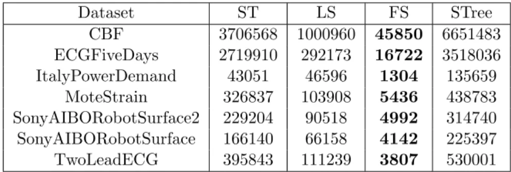
To demonstrate the current run times for the most common shapelet algo-rithms in the literature, seven of the smallest datasets were chosen from the UCR-UEA repository. The results are present in the Table 2.1. In this particular set of experiments, the machine used was a raspberry pi 2. This machine is not designed to run machine learning algorithms in any optimised way. However, with a very lightweight operating system, and controlled environment the timings should be reasonably unbiased. Despite a low-power
machine, the results will all be relative to each other and should give an approximate understanding of the speed of each of the four algorithms. The table demonstrates the speed of the Fast Shapelets algorithm, and is in-line with the claims made in the literature. It was expected that the Shapelet Tree would be the slowest, and that Fast Shapelets would be fastest. With the Shapelet Transform marginally slower than Learn Shapelets. The timings presented were calculated as the average over five runs.
Dataset ST LS FS STree CBF 3706568 1000960 45850 6651483 ECGFiveDays 2719910 292173 16722 3518036 ItalyPowerDemand 43051 46596 1304 135659 MoteStrain 326837 103908 5436 438783 SonyAIBORobotSurface2 229204 90518 4992 314740 SonyAIBORobotSurface 166140 66158 4142 225397 TwoLeadECG 395843 111239 3807 530001
Table 2.1: Timing Results for ST, LS FS and STree in milliseconds.
2.14
Applications of Shapelets
The shapelet approach to time series classification has been applied to numerous problems within the research community. Within the UEA group they have been used on electric device classification, classification of mutant worms and classifying hand outlines [47, 71, 70]. In the original paper the algorithm was applied to leaf outlines [115], further application of the Shapelet Tree algorithm includes gesture recognition [45] and gait recognition [96, 114]. In both of these instances marked improvements were seen from other approaches. In [83] the Fast Shapelets algorithm was used on the outline of horned lizards and turtle skulls, classifying the species and demonstrating the interpretable nature of shapelets on outline problems.
For most of the literature, shapelets or similar motif finding algorithms have been designed and applied to univariate data. The problem of how to handle shapelets in a multivariate domain is an interesting challenge, both in
terms of minimizing workload and producing accurate interpretable results. McGovern et al. [76] applied a similar technique to shapelets on multivariate tornado data, attempting to predict weather patterns. Ghalwash et al. [35] applied shapelets to handle multivariate diagnostic data, which was used for early predictions. The key problems they encountered were dealing with phase independent features across the dimensions which remains an open problem [34].
Shaplet based learning exists outside of classification where examples they have been used in clustering [47, 116, 105] and similar concepts to shapelets were explored in early classification [112, 113, 42, 14].
2.15
Issues With Current Approaches
There a number of issues with the current approaches to shapelet finding and classification. The problems with the shapelet tree were identified and the shapelet transform was proposed as a way of mitigating the issues with embedding the shapelet discovery in a decision tree [70]. There are still a number of issues with the Shapelet Transform, however, which extend to all enumerative shapelet methods. The first major problem is multi class information gain is not very effective at separating one shapelet well from the rest, this is discussed in greater detail chapter 4. The Shapelet Transform still enumerates the entire problem space and on very large datasets such as StarlightCurves full enumeration is still untenable. Logical Shapelets and Fast Shapelets both embed the shapelet discovery and rule implementation in a decision tree. It was shown in [70] the shapelet tree method is significantly worse than a transform based approach and so by extension these methods could benefit greatly from being separate from the classification process. The SAX method for reducing series length in Fast Shapelets smooths the series with PAA. This has the effect of smoothing a series and potentially removing some fundamental shapes within the series. Learn shapelets generates centroids from some initial shapelets and updates them in an online method. The shapelets that are generated as a result of this are often not present in the original dataset, and so lose some of
there interpretability, the runtime is unpredictable because of the learning process. If the algorithm cannot converge a restart and new random shapelets begins the process again. This also means that the memory footprint can be variable.
2.16
Multivariate Time Series Classification
Multivariate time series classification (MTSC) has been gaining traction within the research community. The major issue, until recently, with multi-variate time series analysis is that as the length of the series and the number of dimensions increase they become increasingly difficult to analyse in realis-tic time frames. Whilst this problem may not have been directly solved, as computing power has increased, the ability to work on larger datasets and more complex problems has become easier. Paired with the fact that internet of things (IoT) devices and smart devices are increasingly more common, it means that this type of data is being collected more widely.
One of the major areas of research within MTSC is activity and gesture recognition, otherwise known as human activity recognition (HAR). Gesture and activity recognition is the problem of recognising a particular movement or action within a time series, where the class defining action is potentially phase independent, and the signal to noise ratio is often quite high. The user is potentially performing many different actions, only on
![Figure 2.3: Image taken from Logical Shapelets [79].](https://thumb-us.123doks.com/thumbv2/123dok_us/383219.2542436/32.918.211.704.260.465/figure-image-taken-from-logical-shapelets.webp)