The Classical Hall Effect in Multiply Connected Plane Regions Part II: Spiral Current Streamlines

(1)

ISSN Print: 2327-4352

DOI: 10.4236/jamp.2019.710153 Oct. 11, 2019 2231 Journal of Applied Mathematics and Physics

The Classical Hall Effect in Multiply-Connected

Plane Regions Part II: Spiral Current

Streamlines

Udo Ausserlechner

Department of Sense and Control, Infineon Technologies AG, Villach, Austria

Abstract

Multiply-connected Hall plates show different phenomena than singly con-nected Hall plates. In part I (published in Journal of Applied Physics and Mathematics), we discussed topologies where a stream function can be defined, with special reference to Hall/Anti-Hall bar configurations. In part II, we focus on topologies where no conventional stream function can be defined, like Cor-bino disks. If current is injected and extracted at different boundaries of a mul-tiply-connected conductive region, the current density shows spiral streamlines at strong magnetic field. Spiral streamlines also appear in simply-connected Hall plates when current contacts are located in their interior instead of their boundary, particularly if the contacts are very small. Spiral streamlines and cir-culating current are studied for two complementary planar device geometries: either all boundaries are conducting or all boundaries are insulating. The latter case means point current contacts and it can be treated similarly to singly con-nected Hall plates with peripheral contacts through the definition of a so-called loop stream function. This function also establishes a relation between Hall plates with complementary boundary conditions. The theory is explained by examples.

Keywords

Circulating Current, Corbino Disk, Corbino Images, Corbinotron, Doubly Connected, Hall Plate, Loop Current, Multiply Connected, Non-Peripheral Contacts, Reverse Magnetic Field Reciprocity, Spiral Streamlines, Stream Function

1. Introduction

Part II of this paper largely builds on part I, where we studied the stream func-How to cite this paper: Ausserlechner, U.

(2019) The Classical Hall Effect in Multip-ly-Connected Plane Regions Part II: Spiral Current Streamlines. Journal of Applied Ma-thematics and Physics, 7, 2231-2264.

https://doi.org/10.4236/jamp.2019.710153

Received: August 26, 2019 Accepted: October 8, 2019 Published: October 11, 2019

http://creativecommons.org/licenses/by/4.0/

(2)

DOI: 10.4236/jamp.2019.710153 2232 Journal of Applied Mathematics and Physics

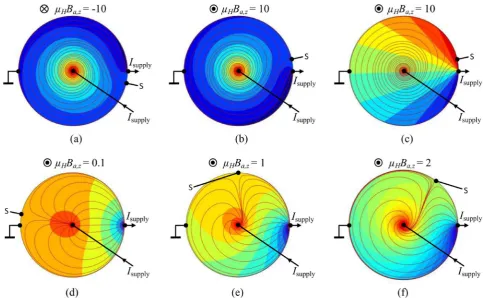
tion of plane multiply-connected Hall plates [1]. In part I, we found that in the absence of spiral streamlines, the stream function obeys particularly simple rules when all boundaries are insulating except for the point-sized contacts. Then the stream function is independent of the applied magnetic field and it is linearly proportional to the Hall potential. Thus, there is no Hall voltage between points on the same current streamline. In the following, we will see that for a large group of Hall plates, no classical stream function exists. As a consequence, such devices show entirely different behavior with the most striking new fea-ture being spiral current streamlines. Such spiral current streamlines were known in multiply-connected Hall plates where all boundaries were contacts [2] [3]. A well-known example of such a topology is the Corbino disk, which max-imizes the magneto-resistance effect. However, there are numerous equivalent shapes—most of them are multiply-connected. This was already known at a very early time [2]. In [3], it was proven that there is no Hall voltage between any contacts of such a device. In [2], the author explicitly states that in such kinds of devices, the equipotential lines remain unaltered by the application of an exter-nal magnetic field. He also gave a general expression for the magnitude of the circulating currents that show up in these devices—we will pick up this thread in Section 3 after some basic definitions in Section 2. In Section 4, we discuss the converse case, i.e., multiply-connected Hall plates with insulating boundaries and point-sized contacts with internal current sources (the case without internal current sources was treated in part I). No theory exists on this kind of Hall plates so far. Finally, Section 5 summarizes all rules of parts I and II for convenient reference. Some symmetries and similarities will become apparent. Appendices A and B give analytical calculations of the current density in singly- and doub-ly-connected regions with insulating boundaries and spiral current streamlines. There, current is injected near the center and flows to a point on the unit circle. Appendix C deals with a specific detail of reverse magnetic field reciprocity for multiply-connected regions in two dimensions.

2. Assumptions and Basic Definitions

In this part II, the same assumptions and definitions apply as in part I [1]. Here we repeat the important ones. We assume only negative charge carriers. Then the Hall effect in a plane Hall plate in the (x, y)-plane with small thickness tH is

described by

(

2 2

)

,

1

H a

H a zB

µ ρ ρµ

ρ µ

− ×

= + × ⇔ =

+

Ε Ε B

E J J B J

(1)

with the externally applied magnetic field

B

a

=

B

a z z,

n

, the specific ohmic

resis-tivity ρ >0_{, and the Hall mobility} µ >H 0. J B× a denotes the vector product

of J and Ba. This work is limited to the linear case, where ρ and µH are

constant versus Ε and Ba. We decompose the potential φ, the electric field

(3)

while changing the polarity of the applied magnetic field.

(

,Ba z,

)

even

(

,Ba z,

)

odd

(

,Ba z,

)

φ r =φ r +φ r (2a)

(

) (

,

) (

,

)

even ,

, ,

,

2

a z a z a z

B B

B φ φ

φ r = r + r − (2b)

(

)

(

) (

,

) (

,

)

odd , ,

, ,

2

a z a z a z H a z

B B

B B φ φ

φ r =φ r = r − r −

(2c)

(

,Ba z,

)

= even

(

,Ba z,

)

+ odd

(

,Ba z,

)

= −∇φ

E r E r E r

(3a)

(

)

(

,

) (

,

)

even , even

, ,

,

2

a z a z

a z

B B

B = E r +E r − = −∇φ

E r

(3b)

(

)

(

)

(

,

) (

,

)

odd , ,

, ,

2

a z a z

a z H a z H

B B

B = B = E r −E r − = −∇φ

E r E r (3c)

(

,Ba z,

)

= even

(

,Ba z,

)

+ odd

(

,Ba z,

)

J r J r J r (4a)

(

)

(

,

) (

,

)

even ,

, ,

,

2

a z a z

a z

B B

B = J r +J r −

J r (4b)

(

) (

,

) (

,

)

odd ,

, ,

,

2

a z a z a z

B B

B =J r −J r −

J r (4c)

The odd potential is also called Hall potential. The difference in Hall potential at two test points on two contacts is called Hall voltage. The odd electric field is also called the Hall electric field. All odd functions vanish at zero applied mag-netic field due to their definition. We denote all even functions at zero applied magnetic fields with an index 0.

( )

,0 even

( )

,0 0

( )

φ r =φ r =φ r (5a)

( )

,0 = even

( )

,0 = 0

( )

E r E r E r (5b)

( )

,0 = even

( )

,0 = 0

( )

J r J r J r

(5c)

In the entire Hall plate, the electric field vectors E are rotated by the Hall an-gle θH against the current density vectors J. From (1), we get

tan

θ

H

=

µ

H a z

B

, .

Inserting (1) for both polarities of the applied magnetic field into (3b, c) and (4b, c) gives relations between even and odd vector fields.

odd = H =ρ odd+ρµH even× a

Ε Ε J J B

_(6a)

even =ρ even+ρµH odd× a

Ε J J B _(6b)

(

)

odd even

odd ₂ ₂

,

1

H a

H a zB

µ

ρ µ

− ×

=

+

Ε Ε B

J

(6c)

(

)

even odd

even 2 2

,

1

H a

H a zB

µ

ρ µ

− ×

=

+

Ε Ε B

J

(6d)

(4)

for a limited class of Hall plates, namely the ones without internal current

sources: 1

z

ρ− ψ

= − ∇ ×

J n holds only if

_

_∫

J n⋅ ds=0 along all loops within the multiply-connected domain (see Section 5 of part I). In this part II, we address Hall plates with internal current sources and therefore we have to use the poten-tial φ_{instead of the conventional stream function}ψ _.

In the stationary case Faraday’s law of electromagnetic induction

t

∇× = −∂ ∂ →E B 0 means that the electric field can be expressed as a gradient of a scalar potential E= −∇φ (cf. (3a)). On the other hand, stationary current flow implies that the amount of electricity entering any volume element inside a Hall plate must equal that leaving it, thus ∇ ⋅ =J 0. Hereby we cut out all current-carrying contacts on the boundaries and inside the Hall effect region (see Section 4). Letting nabla operate on (1) and using these results leads to

0

∇ ⋅E= . It means that under stationary conditions net charge density vanishes everywhere inside a homogeneous Hall plate. From ∇ ⋅E=0 it follows the Laplace equation _∇2_φ₌₀_{for the potential. With (2b, c) also}

even

φ _and φ_H

are solutions of the Laplace equation.

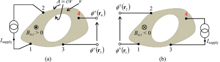
3. Plane Hall Plates Where All Boundaries Are Contacts

On the boundary of a general Hall plate, we distinguish between insulating boundaries and contacts. On the contacts, the value of φ is either forced by ex-ternal voltage sources or it follows from a fixed current into the contact (either

supply

I

±

_{in the supply contacts or zero in the sense contacts). On the insulating}

boundary, there is no normal current density and therefore the electric field is rotated by the Hall angle against the tangent on the boundary. For the potential, this gives an unusual boundary condition ∂ ∂ =φ n

(

tanθH

)

∂ ∂φ t [4]. Here

n

φ φ

∂ ∂ = ⋅∇n means derivation in the direction

n

normal to the boundary and ∂ ∂ = ⋅∇φ t t φ_{means derivation in the direction}t tangential to the boundary with n n⋅ =1, t t⋅ =1, and n t⋅ =0. The magnetic field dependence of the potential enters via

tan

θ

H

=

µ

H a z

B

, in the boundary condition, it does

not enter via Laplace’s equation.

Suppose a Hall plate in two-dimensional space with an arbitrary number of holes. On its outer perimeter and on the hole boundaries it is bounded by con-tacts only, having no insulating boundary. If all concon-tacts are tied to voltage sources, then the boundary conditions contain no magnetic field dependence any more. Thus the electric potential and the electric field in these Hall plates are independent of any applied magnetic field. This means:

0 even even 0

φ φ= =φ ⇒ E =E (7a)

0

H H

φ

⇒ = ⇒ E =0

_(7b)

The Hall potential φH and the Hall electric field EH vanish everywhere in these Hall plates. Inserting (7a, b) into (6c, d) and (1) with E0 ρ =J0 gives:

0

odd 2 2

,

1

H a

H a zB

µ

− ×

= +

J B

(5)

0

even 2 2

,

1

µ

H a zB

= +

J

(8b)

0 0

2 2

,

1

H a

H a zB

µ

− ×

= +

J J B

J

(8c) It holds Jodd = −µHJeven×Ba. In particular Jodd ⊥Jeven and Jeven||J0. We

can solve (8c) for J0. Alternatively, from (7a, b) we can simply say E0=E

and replace E by the left equation in (1). The result is:

0= +µH × a

J J J B

(9a)

Therefore J0 and J are rotated by the Hall angle and scaled in magnitude.

2 2

0 = 1+µH a zB, = cosθH

J J J

(9b) This holds inside the Hall plate but also on the contacts. In other words, at fixed potentials on all contacts, the current density normal to the contacts at the applied magnetic field is smaller by the factor

(

cosθ_H

)

2. We can relate the po-tentials and currents at all contacts of such a Hall plate via a resistance matrix, because the device is electrically linear: due to the superposition principle, the potential at any contact is a linear combination of currents at all contacts. Then

all resistances are proportional to

(

)

2 2 2

,

cosθ_H − 1 µ_{H a z}B

= + _{, which is an even}

function in

B

a z, . Consequently, the Hall voltage vanishes also at constant

supply current of the Hall plate, because it is an odd function in

B

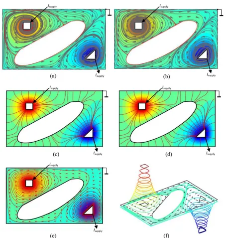
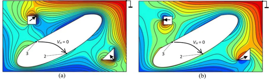
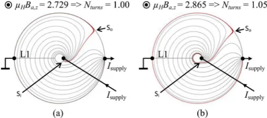
a z, according

to its definition (2c). This is identical to (7b). Zero Hall voltage was shown by Haeusler in his 1967 thesis [3]. With finite element simulations (FEM) it is straightforward to verify this on devices with multiply-connected Hall domains, where all hole boundaries are contacts on different potential. Then the current streamlines show pronounced spirals at large magnetic field (see Figure 1(a) &

Figure 1(b)). However, the vanishing of Hall voltages also holds for geometries where unitary hole boundaries are split in two or more contacts at different po-tential. These cases are extremely challenging to study with FEM, due to insuffi-cient meshing at the interface of contacts on the same boundary.

Furthermore, the electrical equivalent of such a Hall plate with n contacts is a

pure resistor network with resistors

(

)

2

,0 cos

ij ij H

R =R θ between contacts i

and j with 1 ,≤i j n≤ _with i< j_.

R

_ij_,0_{is the respective resistor at zero}

ap-plied magnetic fields. This gives a network with n n

(

−1 2

)

resistors. Hence, the electric response of such a Hall plate with n contacts is fully described by

(

1 2

)

n n− degrees of freedom. This particular group of Hall plates shows sim-ple reciprocity, which means that supply current (input) and sense voltage (out-put) electrodes may be interchanged without any change in the output voltage. Conversely, all other Hall plates show reverse magnetic field reciprocity (RMFR

[5][6][7]), which means that current and voltage electrodes may be interchanged,

(6)

[image:6.595.72.527.63.541.2]

DOI: 10.4236/jamp.2019.710153 2236 Journal of Applied Mathematics and Physics Figure 1. The same Hall effect region as in Figure 9 of part I, but here all boundaries are electrodes drawn as solid black lines. 1 A current is input at the square hole and sunk at the triangular hole. The electrode on the perimeter is grounded for reasons of compatibility with Section 4. (a), (b) Current streamlines and cones in grey, potential in identical color map (red means 25.28 V, blue means −22.07 V) for µH a zB, =10 in (a) and µH a zB, = −10 in (b). The red curve is an equipotential line at 1.2348 V. Note the different directions of the spiral currents in (a) and (b). ((c), (d)) Current streamlines in red, potential in identical color map (red means 0.250307 V, blue means −0.218552 V) for zero applied magnetic field in (c), whereas (d) shows the even current den-sity Jeven and the scaled even potential φeven

(

1+µH2Ba z2,

)

at µH a zB, =10. The plots in (c) and (d) are perfectly identical. (e) The red streamlines and cones denote the odd current density Jodd and the color map is the potential at µH a zB, =10. (f) shows the same data as (e) in a different plot: here the lines and cones denote streamlines and orientation of the odd current density Jodd,

the height above/below the Hall plate and the color-coding denote the potential at µH a zB, =10. Obviously, the streamlines of

odd

J are closed loops, and each loop has a unitary color at constant height, because the Jodd streamlines flow along equipotential

(7)

controlled sources [8][9]. If we supply such a Hall plate with a constant voltage source certain potentials will appear at the other (floating) contacts. If we change the applied magnetic field the ratios of resistances will remain the same and therefore the potentials at the floating contacts will also remain constant.

What happens if we supply the Hall plate with a constant current source in-stead of a constant voltage source? Due to the increase of resistances all poten-tials will rise by the same factor

(

)

2

(

2 2

)

,

cosθH 1 µH a zB

−

= + . The Hall plate

re-sponds as if we would have supplied it with a voltage source whose voltage was increased by the same factor 2 2

,

1+

µ

_{H a z}B _{. With (8a, b) this means:}

odd = −µH 0× a

J J B and Jeven =J0

(10a)

(

2 2

)

even 1 H a zB, 0

φ φ = = +µ φ _and φH =0 (10b)

for constant supply current. The tilde refers to the operating condition “constant supply current” of the Hall plate with conducting boundaries. In words: under constant supply current the even current density is constant versus applied magnetic field and the odd current density is linearly proportional to the applied magnetic field. We will encounter the same behavior of Jodd and Jeven versus

applied magnetic field in Hall plates with all insulating boundaries and point sized contacts with internal current sources (see Section 4). Figure 1(c) & Fig-ure 1(d) show the identities of even current density and even potential with current density and potential at zero applied magnetic field, respectively, ac-cording to (10a, b).

The equipotential lines encircle the current input contact if the contact sub-tends the entire closed boundary of a hole (here we ignore cases where a unitary boundary is split up into several contacts). At zero applied magnetic field, the current density vector is perpendicular to these loops (n J× 0=0), but if a

mag-netic field is impressed on the Hall plate, the current density rotates by the Hall angle while the equipotential line remains fixed at constant supply voltage. Then the component J sinθH is tangential to the equipotential loop. We can

inte-grate this current component along this loop L, which gives the circulation Γ

around the current source.

d sin dH z d

L L L

s θ s s

Γ =

_

_∫

J t⋅ =

_

_∫

J =n ⋅

_

_∫

n J×

(11a) The unit vector t points in tangential direction along the loop L such that the current contact is at its left hand side. The unit vector

n

is orthogonal to the equipotential lines and points away from the current contact. It holds

z× =

n n t. From (8c) we get: 2

0cos θH 0 zcosθHsinθH

= − ×

J J J n (11b)

Inserting (11b) into (11a) with n J× 0=0 gives the circulation:

supply,0 supply

0

cos Hsin H d cos Hsin H tan H

H H

L

I I

s

t t

θ

Γ =

_

_∫

J n⋅ = =

(8)

mag-DOI: 10.4236/jamp.2019.710153 2238 Journal of Applied Mathematics and Physics

netic field

(

)

2

supply supply,0 cos H

I I = θ at fixed supply voltage. In the integration, we used the fact that the total supply current flows out of the closed-loop L. Note that the loop L can be entirely within the conductive region, but it may also comprise portions of electrodes in a multiply-connected Hall plate. In the latter case, the loop enters and leaves the electrode in stagnation points of the current density at zero applied magnetic field (see the red 1.2348 V contour lines in Fig-ure 1(a) & Figure 1(b)). Non-vanishing circulation means that the current streamlines are spirals around the current input electrode whenever there is a closed path around it within the conductive region. The same applies to the cur-rent output electrode (with opposite sign). If the entire outer perimeter is one supply contact, the current pattern has only one spiral pattern, otherwise, it has two spirals in opposite directions. There is no circulation and no spirals around electrodes, where no net current flows in or out. If a floating electrode encircles both current input and output contacts the circulation along it vanishes. Then this loop L can be split up in smaller loops with branching points being the stagnation points of the current density at zero magnetic field, and at least one of these smaller loops has non-vanishing circulation.

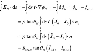
At constant supply voltage, the equipotential lines in the Hall plate are also constant versus applied magnetic field. With (8b) the even current density is or-thogonal to the equipotential lines. With (8a) the odd current density is parallel to the equipotential lines. Thus, Jodd flows in closed loops along equipotential

lines (see Figure 1(e)). Summing up all contributions between two fixed poten-tials φ φ1< 2 at constant supply voltage gives with (8a) the respective circulating

or loop current.

2 2

, 0

loop,12 odd 2 2

1 , 1

2

, 2 1

2 2 sheet 1 , d d 1

d cos sin

1

H a z H

H z

H a z

H a z H

H H

H a z

B t

I t s s

B

B t _s

R B

µ

ρ µ

µ _φ _θ _θ φ φ

ρ µ   = ⋅ = _ × _⋅ + _ _ − = ⋅∇ = +

∫

E

J n n n

t

(12a)

where the unit vector t is tangential to the path, n n tz× = , J0=E0 ρ,

0= −∇φ

E , and Rsheet =ρ tH . Thus, the loop current is finite as long as the

potentials are finite, but it may grow unboundedly if points 1 or 2 are singulari-ties of the potential (e.g. if we force current through the device while the input contact becomes point sized and identical to point 1 or 2. This is similar to Fig-ure 7 in Appendix A). With the equivalent resistor network, it holds:

( )

,0

2 1 supply _cos2 supply

ij ij

H f R

f R I I

φ φ

θ

− = =

(12b) whereby f R

( )

ij is a ratio of polynomials in resistances of the equivalent

resis-tor network. It has the dimension of a resistance. Points 1 and 2 can be inside the conductive region or on the boundary electrodes while the supply current can be injected via the same or via other electrodes. Combining (12a, b) gives:

( )

,0

loop,12 supply sheet tan ij H f R I

(9)

Hence, the loop current can be smaller or larger than the supply current and it grows unboundedly for large Hall angle θH → ±90. For points 1 and 2 being

on electrodes we can compute the loop current without knowledge of the geo-metry or topology, if we only know the equivalent resistor circuit. In Figure 1(e)

for 1 A supply current the circulating current between both supply contacts di-vided by tanθ =H 10 is equal to the supply voltage

φ

2,0

−

φ

1,0

=

4.6886 V

at

zero applied magnetic field divided by the sheet resistance

(

)

loop,12 tan H 2,0 1,0 sheet

I θ = φ −φ R _(for R_sheet= Ω1 _).

(12c) is essentially identical to (7) in [2], however, Green expressed the loop current in terms of the capacitance matrix of the electrode configuration instead of its resistance matrix

R

ij,0.

The expression in (12c) is equal to the number of spiral loops of a current streamline within an annular region bordered by equipotential lines through points 1 and 2 (see also (B6a)).

4. Hall Plates with Point Current Contacts on Different

Boundaries or in Their Interior

In Figure 9 of part I [1], we studied the current pattern and the Hall potential in a rectangular sample with three holes—being square, oval, and triangular—where all boundaries were insulating and both current contacts were on the boundary of the large oval hole. There we noted no current spirals and the current pattern was constant versus applied magnetic field. The Hall voltage between points on the square and on the triangular hole vanished due to the specific locations of these holes. Now we revisit this triply connected Hall plate with insulating boundaries, yet this time we place one point current contact on the boundary of the square hole and the other point current contact on the boundary of the tri-angular hole. The current pattern changes dramatically: Figure 2 shows massive spirals around both holes with current contacts—admittedly this happens only at huge applied magnetic field

µ

H a z

B

,

=

30

(88.1˚ Hall angle). Moreover, in

contrast to part I, the current streamlines are not independent of the applied magnetic field any more: compare the different streamlines in Figure 2(a) &

Figure 2(b) for positive and negative applied magnetic field. However, due to the principle of RMFR ([5][6][7]) there is no Hall voltage between points 2 and 3, which formerly were current contacts in Figure 9 of part I. This holds for ar-bitrary applied magnetic field irrespective of the strength of the spirals (a proof is given in Appendix C). It also holds, if we move the current contacts arbitrari-ly along the boundaries of their respective holes (because in part I the Hall po-tential was homogeneous on all hole boundaries).

(10)

[image:10.595.73.530.61.227.2]

DOI: 10.4236/jamp.2019.710153 2240 Journal of Applied Mathematics and Physics Figure 2. The same Hall plate with insulating boundaries as in Figure 9 of part I [1], but here the point-sized current contacts are at boundaries of different holes: Current is input at point 4 on the boundary of the square hole and sunk at point 1 on the boun-dary of the triangular hole. A point on the perimeter is grounded, but no current flows into this ground node. Both figures show current streamlines in grey color and Hall potential according to the color map (red means 0 V, blue means −30 V): (a) for huge positive magnetic field µH a zB, =30, (b) for huge negative magnetic field µH a zB, = −30. The Hall voltage between points 2 and 3—which were current inputs in Figure 9 of part I—vanishes in spite of the complicated spiral current pattern. The Hall potential along all hole boundaries is not constant. Also, the Hall potential is not constant along the current streamlines. Two arbitrary streamlines are shown in red to guide the eye. They swirl in opposite directions around the current source and their sense of di-rection also changes with the sign of the Hall angle. All displayed quantities were obtained in FEM simulations with COMSOL MULTIPHYSICS in a plane conduction model with (1).

[image:10.595.56.540.369.667.2]

(11)

The leftmost point is grounded. This is similar to a Corbino disk but with point-sized instead of extended contacts. The analytical calculation is done in Appendix A. The figure shows the current streamlines, the potential, and the Hall potential at various magnetic fields as obtained by FEM simulations. Ob-viously, the Hall potential in Figure 3(c) is not constant along the current streamlines and the current streamlines are not constant versus applied magnetic field (compare Figures 3(d)-(f)). The current spiral around the inner current contact is infinitely strong with an infinite circulating current around the point current contact even at very small applied magnetic field (cf. Appendix A).

How can we explain this new phenomenon of spiral current patterns and the fact that current streamlines change with applied magnetic field in contrast to our findings in part I? Apparently, it has something to do with internal current sources. However, there are no spirals if current input and output are on the boundary of the same hole as in Figure 9 of part I. On the other hand, the case of Figure 3 can be regarded as a single point current contact on a hole boundary in the limit of vanishing hole size. Thus the communality is that spiral current patterns are a product of internal hole boundaries being current sources or sinks. In the case of non-zero net current through a hole boundary it is obvious that the stream function ψ_{has a problem, because in Section 5 of part I, we saw}

that ψ _{is constant on insulating boundaries between contacts, and it jumps}

across a contact by the amount of current through the contact (see (18) in part I). If the net current through all contacts on this boundary differs from zero the stream function faces a dilemma: it is forced to change also somewhere in-between two contacts. So the entire concept of a stream function crumbles.

Let us recall from part I that the stream function is proportional to the vertical magnetic field Hz caused by the currents

J J

x

,

y in an infinitely thick Hall

plate with ∂ ∂ =z 0_{. However, a stationary magnetic field due to a current}

makes sense only when this current flows in a closed loop. If the loop is opened, we will have ∇ ⋅ ≠J 0 at its ends and this violates Maxwell’s first law

∇ ×H J= because ∇ ⋅∇ ×H =0. This is explained in [10] and it seems to ad-dress our problem particularly well. In Figure 9(a) of part I, we were inexact, because we did not show the full current loop, i.e., how the current flows from a battery to the current input contact and from the current output contact back to the battery. Yet it is simple to add some curve through the big hole and insert a battery along this path (see Figure 9(b) of part I). Then the Hz field will have

the same value within the hole at the RHS of this curve as it has on the right segment of the hole boundary. Also left of this curve the value of Hz will be

identical to the one on the left segment of the hole boundary (see the blue and red hatched portions of the hole in Figure 9(b) of part I). Hz is discontinuous

on infinitely many points, namely across the current return path. Luckily, these points are outside the conductive region. In these points Hz jumps by

supply H

I

t

. Left and right of the current return path Hz must be constant

(12)

DOI: 10.4236/jamp.2019.710153 2242 Journal of Applied Mathematics and Physics 0

z

∂ ∂ = _{) and there are no currents flowing inside the hole region except along}

the arbitrary current return path. Also in Figure 6 and Figure 7 of part I, we can close the current loops—there they can be closed outside the perimeter of the conductive regions. Therefore they add constant Hz outside the conductive

re-gions. Hence, we did not miss these return paths when we discussed the stream function inside the conductive region. Finally, apart from the current return path—ψ is constant outside the conductive regions and inside the holes, and this agrees with the familiar notion J =0 there. In fact, this is even a simple explanation why ψ is constant on a hole boundary without current contacts: it is constant there because inside the entire hole Hz =constant because no

cur-rent flows inside the hole region.

The situation is different in Figure 2 and Figure 3. There we cannot close the current loop without cutting through the conductive region. We cannot solve this problem by pulling current straps out of the (x, y) drawing plane because the Hall plates are supposed to be infinitely thick for our Hz versus ψ analogy in

part I [1], we are not allowed to work with 3D tricks in a 2D world. Hence, the return current path goes right through the conductive region and this will affect

z

H and ψ there, too. Such a return current sheet will make Hz

disconti-nuous at infinitely many points in the conductive region.

On the other hand, ignoring the current return path altogether gives wrong results for Hz and ψ, as the following example illustrates. Suppose an

infi-nitely long hollow cylinder along z-direction. The cylinder consists of poorly conducting material like most high mobility semiconductors. No magnetic field is applied. The cylinder bore is clad with a perfectly conducting contact and also the outer surface is clad with the same material. If we tie one contact to ground and apply a voltage to the other contact a radial current density will result

1

r r−

∝

J n . This is an infinitely thick Corbino disk at zero applied magnetic fields. What is the magnetic field generated by the current density? Solving Maxwell’s first equation ∇ ×H J= gives H n= zarctan

(

y x

)

, but also H = −nzarctan

(

x y

)

is a solution. Thus, the solutions are discontinuous on x- and y-axes, respectively, and the solution is not even unique. Moreover, from physical intuition, we can consider a thin circular disk with radial current density. It will have only azimu-thal magnetic field: CW above its top surface and CCW below its bottom surface. If we pile up an identical second circular disk the azimuthal fields of both disks cancel at their interface. Piling up infinitely many of them will cancel out the field in all test points. In the end, there is no (!) magnetic field caused by this current distribution—which of course contradicts Maxwell’s first equation

(13)

To sum up, there exists no stream function, if the electrodes in a 2D conduc-tion problem are placed in such a manner that the current return path via the battery cuts through the conductive region. If both supply contacts are on the same boundary we can add a current return path outside the conductive region or inside a hole. Then the current density is equal to the curl of a unique mag-netic field perpendicular to the plane of conduction. This is the stream function. It is continuous in nearly all points, i.e., in all points with exception of a finite number of points (namely a finite number of point supply contacts on the boundaries). Then we can interpret ψ as a current potential function. Conversely, problems like in Figure 2 and Figure 3 have internal current sources, i.e., single supply contacts on boundaries or within the conductive region. For them, we cannot close the current loop outside the conductive region or inside a hole in a 2D analysis. These current patterns are not identical to the curl of a unique ver-tical magnetic field.

In order to reconcile ∇ ⋅ ≠J 0_{with Maxwell’s first law} ∇ ×H J= we may add an extra current density Je (inside the Hall effect region, not outside)

which closes the current loop. From Maxwell, we know that every closed current loop is accompanied by a magnetic field H, whereby the current density is the curl of H.

e e

∇×H J J= + ⇒ ∇ ⋅ = −∇ ⋅J J

(13) Note that Je may be a continuous function (as below in (14a)) or a

discon-tinuous current return sheet (as in Figure 7(b) and Figure 9(b), both in part I

[1]). In both cases, the Hz-component has the physical meaning of a magnetic

field generated by J J+ e and with (11) in part I the stream function also

speci-fies J J+ e via J J+ e = −ρ−1∇ ×ψnz. Of course, this procedure helps us only

in the calculation of the current pattern J J+ e and not for the original J. But

if Je is known a priori, we can simply subtract it from J J+ e to get J . In

the following, we will use Je which is not known a priori, but which has a

cer-tain relation to J. This will help us to break up the original problem into smaller sub-problems by decomposition of J into Jeven and Jodd.

If we choose Je= −J B

(

− a

)

, contacts connected to current sources are no

sources for the J J+ e vector field, although they are sources for the J vector

field. Therefore we may write according to (8) in part I and with J J+ e =2Jodd.

odd d 0 odd z,odd z

C

s H

⋅ = ⇒ = ∇×

∫

J n J n



(14a)

The meaning of (14a) is: Since Jodd is a vector field free of sources, its flux

through any closed contour C in the multiply-connected Hall plate vanishes, and therefore Jodd can be expressed as the curl of a magnetic field

H

z,odd

n

z. The

label

H

z,odd is used to discriminate it against Hz in part I [1]. (14a) holds for

Hall plates with both point-sized and extended contacts. With (14a) we can de-fine a so-called loop stream function

ψ

loop analogous to the conventional

stream function ψ of part I.

loop

H

z,odd

(14)

Analogous to part I,

ψ

loop is constant along the streamlines of Jodd, and

therefore

J

odd

⋅∇

ψ

loop

=

0

. Without internal current sources—like in part I— loop

ψ

vanishes because then the current density is independent of the applied magnetic field: J B

( )

− =J B

( )

⇒Jodd =0. The definition implies that

ψ

loop is

an odd function of the applied magnetic field. Hence,

ψ

loop depends on Ba

whereas ψ in part I was constant w.r.t. Ba. Jodd is linked to Hodd via (14a)

and therefore ∇×Jodd =0. Hence

ψ

loop fullfills the Laplace equation and it is

constant on all boundaries without current contacts, because there is always a

odd

J -streamline that flows along such a boundary. If we insert (1) into (3c), we get with (2a-c) and (14a, b):

(

2 2

)

, even 1 , loop

H z H a zB H a zB

φ µ φ µ ψ 

∇ = − ×n _ ∇ + + ∇ _

(15a)

These are the Cauchy-Riemann differential equations. It means that the function

(

2 2

)

, , , even 1 , loop

R H I H H H a z H a z

F _{= −}iF ₌φ ₊iµ B φ _{+ +}µ B ψ 

  (15b)

is analytical. We call it the complex Hall potential

F

R H, because its real part is

the Hall potential φH, whereas the complex potential FR in (21) of part I has

the potential φ_{as its real part. (15b) differs from}

F

_R_,odd in (22) of part I only in the term with the loop stream function. Therefore (15b) is a generalization of (22) in part I, because

ψ

loop was zero there. Hence, both FR H, and

F

R,odd are

odd in

B

a z, . (15a) is equivalent to

(

2 2

)

, even 1 , loop

z×∇φH =µH a zB ∇φ + +µH a zB ∇ψ

n . (15c)

If we integrate the odd current density Jodd traversing a contour (extruded

into thickness direction) that starts at point 1 and ends at point 2 we get with (14a, b).

2 2

loop,12 odd loop

1 1

2

loop,1 loop,2

loop

sheet 1 sheet

d d

1 d

H

H t z

I t s s

s

R R

ψ ρ

ψ ψ

ψ

= ⋅ = ⋅ ×∇

− −

= ⋅∇ =

∫

J n n n

t

(16)

If points 1 and 2 are left and right of a point current contact on a boundary, it holds

∫

₁2J B n

( )

a ⋅ ds=

∫

₁2J B n

(

− a

)

⋅ ds. Inserting this into (16) shows that

ψ

loop

is also continuous on boundaries with point current contacts, whereas in part I

ψ was discontinuous there. On extended contacts

ψ

loop has identical values at

both ends, but it varies along the contact. If points 1 and 2 in (16) are point supply contacts on different boundaries,

I

loop,12 is the total circulating current

that flows in the Hall plate. It can be smaller or larger than the supply current and it can even become infinite (see Appendix A). In the absence of internal current sources, i.e., when both point supply contacts are on the same boundary, the circulating current vanishes, because then the loop stream function vanishes. If we use Maxwell’s law in the quasistatic case

_

_∫

E s⋅d =0 at positive and neg-ative applied magnetic field and subtract both equations it gives



∫

EH⋅ds=0

(see (3c)). Inserting (1) gives the circulation Γ_{of the odd current density} J_odd

(15)

(

)

odd , even

supply

, even odd ,

d d

d H a z

C C

H a z H a z

H C

B s

I

B s B

t µ

µ µ

Γ = ⋅ = ⋅

= + ⋅ =

∫

J s J n

J J n



(17a)

In (17a), we were allowed to add Jodd in the integrand because integration of odd⋅

J n over a closed path gives zero according to (16). The circulation of a specific pattern of spiral current streamlines is computed in Appendix A. Note that the circulation in (17a) is identical to the circulation in Hall plates where all boundaries are contacts (see (11c)). On the other hand, if we use



∫

Eeven⋅ds=0 and (1) and (14a, b) it follows:

even d 0

C

⋅ =

∫

J s



(17b) With J J= even+Jodd and (17a, b), it is clear that the circulation of J is

equal to the circulation of Jodd. Spiral current streamlines appear only for

odd ≠

J 0. Therefore we have no spirals in the absence of internal current sources like in part I [1], where it holds Jodd =0 (because J was independent of Ba).

Conversely, in the case of internal current sources there are also no spirals at

a=

B 0. Thus, it needs applied magnetic field and internal current sources to produce circulating current. Thereby it is irrelevant if the internal current sources are embedded in the conductive region or if they are on boundaries of holes in the conductive region. The method of Corbino images from [13] is also a way to prove that the circulation around single point contacts is given by (17a) and that it vanishes when both supply contacts are encircled. In [13] this method was used for conductive regions with one boundary, but it can also be genera-lized for more boundaries (like ring domains) if one uses a superposition of infi-nitely many images [14][15].

Inserting the right hand sides of (3b, c) into (6d) and eliminating the vector product by use of (15c) gives:

(

)

even =−_ρ1∇ φeven+µH a zB,ψloop

J

(18) In (18), the terms in the brackets act like a potential, which fulfills the Laplace equation because of 2

even 0

φ

∇ = and 2

loop 0

ψ

∇ = _{. On the boundary}J_even⋅n

is given – it is zero at the insulating boundary and it is a Dirac delta pulse of strength

±

I

supply

t

H at the point-sized supply contacts. However, −ρJeven⋅n

is the normal derivative of the bracket term in (18), which is a von Neumann boundary condition that does not depend on the applied magnetic field. There-fore the term in the brackets of (18) does not depend on the applied magnetic field. Yet, at

B

a z,

=

0

it is equal to φ0 (up to an arbitrary additive constant)

and therefore

0 even H a z

B

, loop

φ φ

=

+

µ

ψ

_.

(19) In (19), we implicitly assume the arbitrary additive constant in

ψ

loop such

that

ψ

loop

=

0

in the ground node where it holds φ0=φeven =0. On the other

(16)

odd

J . Since Jodd vanishes outside the perimeter of the Hall plate, also

,odd

0

z

H

=

_{there. Therefore}_{we have to ground a point on the perimeter of the}

multiply-connected Hall plate. (19) in (18) with E0 ρ =J0 gives:

even = 0

J J ₍₂₀₎

which is identical to (10a) in Section 3 (both times the Hall plates are supplied by constant current sources). (19) can be seen as an alternative definition of the loop stream function, being the negative increase in even potential divided by

,

H a z

B

µ

_{. Since}

ψ

_loop_{does not change along any hole or perimeter boundaries,}

even 0

φ −φ _{is also homogeneous there according to (19). With (19) we can}

elimi-nate the even potential in (15b).

(

)

, , , 0 loop

R H I H H H a z

F = −iF =φ +i µ B φ ψ+

(21a)

(

, 0 loop

)

H z H a zB

φ µ φ ψ

∇ = − ×n ∇ + ∇ (21b) Curves of constant Hall potential are orthogonal to curves of constant

, 0 loop

H a z

B

µ

φ ψ

+

.

Next, we compute the Hall electric field perpendicular to an insulating boun-dary from (6a) with Jodd⋅ =n 0 and with (20).

, 0 , 0

H

H H _n H a zB z H a zB

φ

φ −∂ ρµ ρµ

⋅ = − ⋅∇ = = × ⋅ = ⋅

∂

E n n J n n J t

(22) Thus, the Hall potential is a harmonic function, which satisfies von Neumann boundary conditions with values that are linearly proportional to applied mag-netic field. Therefore φH is perfectly linear in

µ

H a z

B

, (the same applies to

Hall plates with insulating boundaries and point-sized contacts without internal current sources, see part I [1]). With (21a, b) it follows that

ψ

loop is also

per-fectly linear in

µ

H a z

B

, . Therefore, also Jodd is linear in

µ

H a z

B

, (see (14a,b)).

Consequently, the total current pattern J J= 0+Jodd is not constant versus

applied magnetic field – which is in contrast to the Hall plates discussed in part I. Therefore, in the case of internal current sources the current density depends on the applied magnetic field even if the contacts are only point-sized. This explains the different streamlines at positive and negative magnetic field in Figure 2(a) &

Figure 2(b). At positive Hall angle they go counter-clockwise (CCW) around the current input at the square hole and clockwise (CW) around the current sink at the triangle. At negative Hall angle the directions of the spirals are inverted.

From (19) it follows that φeven−φ0 is proportional to the second power of ,

H a z

B

µ

_{. In other words,}

₍

₎

₍

₎

2

even 0 H a zB,

φ −φ µ does not depend on the applied

magnetic field, and since it is equal to ψloop

(

µH a zB,

)

it is constant on all boundaries. Moreover,

(

φeven−φ0

)

(

µH a zB,

)

2 is a solution of the Laplace equa-tion. Consequently, ψloop

(

µH a zB,

)

is linearly proportional to the potential φ0 of the very same Hall plate with the same supply current into the same supply current contacts but all boundaries are conducting (like in Section 3) instead of insulating.

loop c1 H a zB, 0

ψ

=

µ

φ



(17)

In (23a), we chose the arbitrary additive constant of φ0 being a solution of the Laplace equation such that φ0=0 where

ψ

loop

=

0

, i.e., the electrode being

the perimeter must be grounded. The constant c1 follows from the circulation.

Inserting (23a) into (17a) gives:

0

odd 1 ,

supply

1 0 1

H

d d

tan d tan

t H a z

C C

H H

C

c B s

I

c s c

φ µ

ρ

θ θ

∇

Γ = ⋅ = ⋅

= − ⋅ = −

∫

J s n

J n





(23b)

Setting this equal to (11c) gives:

1 1

c = − _(23c)

(23a, c) relate the loop stream function in a multiply-connected Hall plate with insulating boundaries to the potential at zero applied magnetic field in the same Hall effect region, yet with all boundaries being electrodes. Therefore, on the contacts

ψ

loop is a function of the resistors

R

ij,0 of Section 3. We do not

even need to know the geometry of the Hall plate to compute it—it already fol-lows from the equivalent resistor circuit

R

ij,0 at zero applied magnetic field for

the Hall plate with all boundaries being contacts. Inserting (23a) into (16) with points 1 and 2 being negative and positive supply contacts, respectively, and comparing to (12c) proves that the total circulating current is identical in two identical Hall regions with (i) point sized contacts with insulating boundaries and (ii) all boundaries conducting, provided the same supply current is injected.

Inserting (23a) into (21a) gives:

(

)

, , , 0 0

R H I H H H a z

F = −iF =φ +i Bµ φ φ− 

(24) Thus, the lines of constant Hall potential are orthogonal to the lines of con-stant φ φ0− 0. Therefore, the Hall voltage vanishes, if it is sampled between two points on the same streamline of the current vector field J0−J0, whereby J0

is the current density of the Hall plate with all boundaries being insulating and 0

J is the current density of the Hall plate with all boundaries being electrodes, and both Hall plates are supplied with the same fixed current at zero applied magnetic field.

Inserting (23a, c) into (14a, b) shows that at fixed supply current the odd cur-rent density in the Hall plate with insulating boundaries is identical to the odd current density in the same Hall effect region with all boundaries being electrodes.

0

tan odd = odd = θH z×

J J n J ₍₂₅₎

With (20) and (25) we can express even and odd current densities and electric fields via J0 and J0, so that from now on we would not need

ψ

loop any more.

(

0 0

)

tan

H =ρ θH − × z

E J J n (26)

(18)

(

)

(

)

(

)

2 2 2

,1 ,2

1 1 1

2

0 0

1 2

0 0

1

sheet 0,12 0,12

d d d

tan d

tan

H H H H H

H z

H

s

R I I

φ φ φ φ

ρ θ

θ

⋅ = − ⋅∇ = − = −

= ⋅ − ×

= − ⋅

= −

∫

E s t

t J J n

J J n



(27a)

where I0,12,I0,12 are the currents flowing across a contour that connects points

1 and 2. Thereby the applied magnetic field vanishes and all boundaries of the Hall plate are electrodes (for I0,12) and insulating (for

I

0,12), respectively.

The-reby the same supply current flows into the same boundaries. Analogous to (7) and (19) in Part I, we can write for the Hall voltage between arbitrary points 1 and 2

,12 supply sheet ,12

tan

H H H

V

=

I

R G

θ

(27b) with the Hall geometry factor

0,12 0,12 ,12

supply

H

I I

G

I

− = 

(27c) Thus, the Hall geometry factor is again (like in part I) a ratio of a current flowing across a contour connecting the two point-sized output contacts over the supply current, however, here we have I0,12−I0,12 in the numerator,

whe-reas we had

−

I

12

= −

I

0,12 in part I. Note that in part I point-sized current input

and output contacts were at the same boundary, which means I0,12 =0, because

the electrode on that boundary is a perfect short. Therefore, (27c) is a generali-zation of (19) in part I. If the points 1 and 2 are on the same boundary the cur-rent I0,12 goes continuously to zero as the two points approach, whereas the

current

I

0,12

=

I

supply if a supply contact is between points 1 and 2. This means

that along boundaries the Hall voltage jumps abruptly across point current contacts and it varies smoothly on the rest of the boundary. Due to the subtraction in (27c) the Hall voltage along boundaries is smaller in the case of spiral current streamlines than in the absence of internal current sources like in part I. (27b, c) also show that locations of zero Hall voltage do no change versus applied magnetic field.

[image:18.595.278.465.72.175.2]

A comparison of this section with the preceding one shows that the Hall elec-tric field in multiply connected Hall plates vanishes everywhere if all boundaries are highly conducting, whereas it is proportional to the applied magnetic field everywhere if all boundaries are insulating.

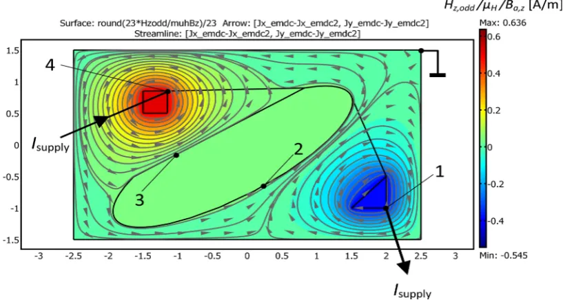
Figure 4 shows the spiral current streamlines and the loop stream function for the Hall plate of Figure 2 with the same current supply contacts: Jodd flows in

closed loops around the current contacts while

ψ

loop is constant on these loops.

Thus

ψ

loop is also constant on all hole boundaries and zero on the outer

boun-dary, just as we would expect it for the vertical magnetic field

H

z,odd generated

by a current vector field Jodd according to (14a). Figure 5 shows that φeven−φ0

(19)

[image:19.595.93.502.72.290.2]

DOI: 10.4236/jamp.2019.710153 2249 Journal of Applied Mathematics and Physics Figure 4. The same Hall plate with insulating boundaries as in Figure 2, with the same supply current of 1 A into the same point current contacts 4 and 1. The grey lines are streamlines of Jodd. They are not spirals, but closed loops around the holes with the

current contacts. The grey cones denote the orientation of Jodd. The color-coding denotes the magnetic field Hz odd, in A/m normalized by µH a zB, . All results are obtained by three coupled FEM calculations with COMSOL MULTIPHYSICS: two are conductive media calculations with the conductivity tensor from (1) for positive and negative applied magnetic field

, 10

H a zB

µ = ± . The resulting current density for positive magnetic field is denoted by the components Jx_emdc, Jy_emdc. The re-sult for negative magnetic field is Jx_emdc2, Jy_emdc2. Half the difference of current densities in these two calculations is set equal to J_odd=

(

Jx_emdc-Jx_emdc2

)

n_x 2 Jy_emdc-Jy_emdc2+

(

)

n_y 2. The third calculation computes the magnetic field Hz odd, in response to Jodd, whereby the boundary condition was “electric insulation” (Hz odd, =0) on the outer boundary. The current streamlines are identical with the contour lines of Hz odd, . The hole boundaries are also contour lines of Hz odd, with values of 6.36, 0.24, −5.45 A/m for the square hole, the large hole, and the triangular hole, respectively. Inside the holes the Hz odd, -field is homogeneous. No current flows into the ground node on the perimeter.

Figure 5. The same Hall plate with insulating boundaries as in Figure 2 and Figure 4, with the same supply current of 1 A into the same point current contacts 4 and 1. The geometry is drawn in black lines. The color lines denote the function

(

0

)

(

,

)

loop even HBa z

ψ φ φ µ

− = − where blue means negative, green means zero, and red means positive (the precise values are given as labels). The height above/below the Hall plate also denotes

(

φeven−φ0

)

(

µHBa z,

)

. Evidently, the hole boundaries and the perimeter

[image:19.595.192.407.479.619.2]

(20)

[image:20.595.84.539.73.209.2]

DOI: 10.4236/jamp.2019.710153 2250 Journal of Applied Mathematics and Physics Figure 6. The same Hall plate with insulating boundaries as in Figure 2, Figure 4 and Figure 5. The grey streamlines denote J J0−0 and the color map gives the Hall potential at µH a zB, = ±10 (red means 0 V, blue means −10 V). (a), (b) different point current contacts on the same hole boundaries. The supply current is 1 A. The ground node is a point on the perimeter. No current flows into this ground node. Obviously, the streamlines are identical with equipotential lines of the Hall potential. The Hall voltage between points 2 and 3 vanishes due to RMFR, because they were current contacts in Figure 9 of part I [1] while the boundaries of the square and triangular holes were on the same streamline of J . There-fore, the color map has identical color at points 2 and 3. The results are obtained by four conductive media FEM calcula-tions with COMSOL MULTIPHYSICS with the conductivity tensor from (1) for µH a zB, = ±10 and µH a zB, =0 first with insulating boundaries and then with all boundaries being electrodes.

Finally, we briefly mention that there are alternative ways to tackle the prob-lem of Section 4. Instead of the loop stream function, one could also define a generalized stream function Ψ with:

0 0 _ρ z

Ψ − = −∇ ×

J J n

(28) because



∫

(

J0−J0

)

⋅nds=0 for all closed paths in a multiply-connected 2D Hall effect region (compare with (8) in part I). Inside the Hall effect region, it

holds

(

)

1

(

2 2

)

0 0 ρ− φ0 φ0 0

∇ ⋅ J −J = − ∇ − ∇  = . Ψ_{does not depend on the}

ap-plied magnetic field. Then we get with (26):

tan

H H

φ = − θ Ψ

₍₂₉₎

where we define Ψ=0_{in the ground node. These equations have greater}

simi-larity to (13) and (17a) in part I.

5. A Summary of Simple Rules

In parts I and II, we derived simple rules to understand the classical (non-quantum) Hall potential in thin, plane and homogeneous regions with linear material properties. Here we compile them.

(21)

of the current density can be obtained from a loop stream function. Stream function and loop stream function can be interpreted as the vertical component of a magnetic field generated by the respective current in the Hall plate with in-finite thickness.

Without internal current sources and when all boundaries are insulating (apart from point sized current contacts) the current density is constant versus changes in applied magnetic field. The Hall potential is constant along all cur-rent streamlines. Since any closed boundary (hole boundary or perimeter) with-out current contacts is encircled by a single current streamline, the Hall potential is constant on the boundary. Therefore, the Hall voltage between any two points on such a boundary vanishes. In all test points, the Hall potential is linearly proportional to

µ

H a z

B

, . The Hall voltage between any two points is

propor-tional to the current flowing across a contour between both points.

If there are no current sources in the Hall plate but at least one contact is ex-tended, the current density changes versus applied magnetic field. Then, in gen-eral, the Hall voltage between two points on the same boundary does not vanish, even if that boundary has no current contacts. The Hall voltage is not strictly li-near versus applied magnetic field. At very large Hall angles extended contacts become similar to point-sized contacts located at one of both ends of the ex-tended contacts—which one depends on the polarity of the applied magnetic field. Therefore, at very large Hall angles the Hall voltage diminishes if it is tapped between points with no current flowing in-between (e.g. on hole bounda-ries with no contacts).

If the peripheral boundary and all hole boundaries of a multiply-connected Hall plate are electrodes there is no Hall voltage between any points (or contacts) of the Hall plate. The device acts like a network of resistors, whose resistances are proportional to 2 2

,

1+

µ

H a zB . This is the only case when a Hall plate is

reci-procal instead of reverse magnetic field recireci-procal.