Abstract — Power maximization approach is applied for dynamical chemical engines and static solid oxide fuel cells (SOFC) treated as power generators. Performance curves of a dynamical chemical engine and a static SOFC system are analyzed. Hamiltonian based algorithm is displayed and applied in optimization of static and dynamic models. Dynamic chemical engine is optimized subject to the period constraint and criterion of total power produced. Also, a steady state model of a high-temperature fuel cell is optimized, which refers to constant chemical potentials of incoming hydrogen fuel and oxidant. Lowering of the cell voltage below its reversible value is attributed to polarizations (activation, concentration and ohmic) and imperfect conversions of reactions. Power formula subsumes effects of efficiency, transport laws and irreversible polarizations. The reversible electrochemical theory is extended to the cases of efficiency lowering; these cases include systems with reduced affinities and an idle run voltage. Optimum conditions are found for definite currents. Power data differ for power generated and consumed, and depend on system’s characteristics (current intensity, mass transfer coefficients, polarization, electrode surface area, etc.). They provide bounds for power generators, which are more exact and informative than classical reversible bounds for the chemical or electrochemical transformation.
Index Terms—Keywords. Resources, chemical efficiency, electrochemical efficiency, entropy production, engines.
I. INTRODUCTION
Limited amount or flow of resources working in engines causes lowering of resource potentials in time (chronological or spatial). Consequently, all studies of the resource downgrading in engines apply the methods of dynamic optimization [1]. From the optimization viewpoint, dynamical process is every one with sequence of states, developing either in the chronological time or in (spatial) holdup time. The first group refers to unsteady processes in non-stationary systems, the second group may involve steady state systems.
Approaches of finite rate thermodynamics to power systems lead to solutions which describe various forms of limits on power and energy generation (consumption), including, in the dynamical cases, finite-rate extensions of standard availabilities [1].
In this research we treat power limits in (static and dynamical) chemical or electrochemical power systems driven by fluids that are restricted in their amount or magnitude of flow, and, as such, are the system resources. A Manuscript received October 25, 2010. This research was supported by the grant: Thermodynamics and Optimization of Chemical and Electrochemical Energy Generators with Applications to Fuel Cells, nr N N208 019434, from The Polish Ministry of Science. S. Sieniutycz is with the Faculty of Chemical and Process Engineering at Warsaw TU, 1 Waryńskiego Street, Warszawa, 00645 Poland (phone: 00-48228256340; fax: 00-48228251440; e-mail: sieniutycz@ ichip.pw.edu.pl).
power limit is an upper (lower) bound on power produced (consumed) in the system. A resource is a valuable substance or energy used in a process; its value is often quantified by specifying its exergy, a maximum work that can be obtained when the resource relaxes to the equilibrium. Reversible relaxation of the resource is quantified by the classical exergy. When dissipative phenomena prevail, generalized exergies play a role. In fact, generalized exergies quantify deviations of the real system’s efficiencies from the perfect (reversible) efficiencies.
An exergy type function is obtained as the standardized potential which is the component of solution to the variational problem of extremum work under suitable boundary conditions. Other components of the dynamic solution are optimal trajectory and optimal control. In purely thermal systems (those without chemical changes) the trajectory is characterized by temperature of the resource fluid, T(t), whereas the control is Carnot temperature T’(t) defined in our previous work [1, 2]. For chemical and electrochemical systems Carnot chemical potential(s) µ’k(t) also play a role. Whenever T’(t) and µ’k(t) differ from T(t) and µk(t) the resource relaxes with a finite rate, and with an efficiency vector different from the perfect efficiency. Only when T’ = T and µ’k(t) = µk(t) the efficiencies are ideal, but this corresponds with an infinitely slow relaxation rate of the resource (for example the resource relaxation to the thermodynamic equilibrium with the fluid of the lower (second) reservoir). The concept of Carnot controls can be applied to both static and dynamical power systems working in quite diverse configurations.
The structure of this paper is as follows. Section II displays a canonical Hamiltonian algorithm which is particularly suitable for dynamic problems of power optimization. Basic properties of steady chemical generators are recalled in Sec. III, and their theory is extended to dynamic systems in Sec. IV. Section V presents a discrete optimization algorithm for a dynamical chemical engine. Power outputs of steady-state electrochemical engines (fuel cells) are analyzed in Sec. VI. A theoretical assessment of limits on real power yield in thermo-electrochemical systems is presented in Sec. VII. Section VIII summarizes main findings of the paper.
The size limitation of our paper does not allow for inclusion of all derivations to make the paper self-contained, thus the reader may need to turn to some previous works, [1] - [6].
II. HAMILTONIAN ALGORITHMS
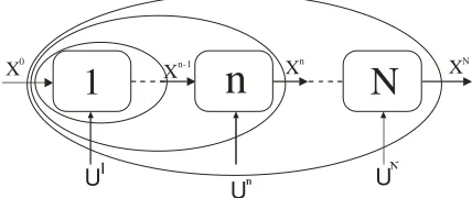
The dynamic changes for the discrete state of a multistage system can be described by a set of ordinary difference equations called the state transformations which describe the discrete state Xn = (xn, tn) from the stage n-1 in terms of the
Maximizing Power Generation in Chemical
Systems and Fuel Cells
state from the stage n and some control variables Un. Fig.1 illustrates the corresponding block scheme.
1
n
N
X0 Xn-1 Xn XN
U
[image:2.612.76.290.84.174.2]U U
Figure 1. A block scheme of general dynamical process.
The set of discrete state transformations can be written in the following general form
(
)
1
, ,
n n n n n
t
− =
x T x U (1)
and
1
n n n
t − t θ
= − , (2) where Xn = (xn, tn) and n
(
n, n)
θ =
U u is an enlarged vector of control variables which includes the discrete interval of time
θ
n, and the time variable tn is identified with any state variable growing monotonically. After defining the functionn n n n n n
n (x T (x ,t ,U ))/θ
f = − (3)
the above state transformations can be transformed into the form [7, 8]
xn−1=xn−fn(xn,tn,un,
θ
n)θ
n (4) andn n n
t
t −1= −
θ
(5) As they involve the discrete rates (fn,1), we call this form the “standard form”.A performance index describing a generalized profit is in this formalism (total power in our case) is defined by the following equation
n n n n n n
N
n N N
t f W
P 0(x , ,u ,
θ
)θ
1 =
∑
=
≡ & (6) where f0 is the generation rate for the generalized profit (power in the case of energy yield problems). To solve the optimization problem of extremum W, a (enlarged) Hamiltonian is defined in the following form
1 −
1 =
1 − 0
1 − 1
−
+ +
≡
∑
nt s
i
n n n n n i n i n n n n n
n n n n n n
z t
f z t
f t H
) , , , ( )
, , , (
) , , , , ( ~
θ θ
θ
u x u
x
u z x
(7)
where zi are adjoint (Pontryagin’s) variables [1].
In an optimal process the enlarged Hamiltonian H~n−1 satisfies in the enlarged phase space x = (x, t) and z = (z, zt) the following equations:
1 −
1 − 1
−
∂ ∂ = −
n i
n
n n i n i
z H x
x ~
θ (8)
(state equations) and
n i n
n n i n i
x H z
z
∂ ∂ − =
− −1 ~ −1
θ (9) (adjoint equations), and the equations which describe the necessary optimality conditions for decision variables un. For example, if the optimal control lies within an interior of admissible control set
0 = ∂
∂[θnH~n−1
(
xn,zn−1,θn,un)]/ θn (10)and
0 = ∂
∂ −1
n j n
u H~
(11) [7, 8]. Equation (10) implies constancy of the enlarged Hamiltonian along a discrete optimal path whenever discrete rates fi are independent of θn
. In addition, the energy-like Hamiltonian (without zt term) is constant for the process whose rates are independent of time tn. Under the convexity properties for rate functions and constraining sets the optimal controls are described by the following equations
)} , , , ( ~ { max
arg n n n n n n
n H z
n
θ θ
θ
θ
u x −1 1
−
= (12)
and
)} , , , ( ~ { max
arg n n n n n
n H z
n
θ u x
u u
1 − 1 −
= (13)
(n=1,...N; i=1,...s+1 and j =1,...r.) Optimization theory for generalized (θθθθn
-dependent) costs and rates [7,8] provides the bridge between constant-H algorithms [9,10] and more conventional ones such as those by Katz [11], Halkin [12], Canon et al. [13], Boltyanskii [14], and many others. Since, as shown by Eq. (10), control θn
can be included in the Hamiltonian definition, i.e. an effective Hamiltonian can be used Hn-1= n−1
H~ θn, extremum conditions (8)-(13) can be written in terms of Hn-1. The related canonical
set is that of Halkin
1 1 1
− − −
∂ ∂ =
− n
i n n i n i
z x
x H (14)
n i n n
i n i
x z
z
∂ ∂ − = −
1 − 1
− H
(15) [12]. Qualitative difference between the role of controls un and θn
in the optimization algorithm is then lost since they both follow from the same stationarity condition for Hamiltonian Hn-1in an optimal process. For example, in the weak maximum principle
0 = ∂ ∂ = ∂
∂ −1 −1
n j n
n n
u
H H
in agreement with Eqs. (10) and (11) above. Moreover, Eq. (16) implies the necessary condition (10) if the discrete model is independent of time interval θ.
To date Hamilonian algorithms were used in power systems for models with θ- independent discrete rates [15]. Yet, Poświata and Szwast have shown many their applications in
exergy optimization of thermal and separation systems, in particular fluidized dryers [7,16]. Sieniutycz has shown some other applications for energy and separation systems and for a minimum time problem [8]. In view of diversity of discrete rates, which may contain explicit time intervals θ as the consequence of various ways of discretizing, applications of algorithm (4) - (13) in power or separation systems may be quite appropriate and useful. In particular, the algorithm is suitable in numerical studies of the optimal solutions for the discrete equations of the unsteady chemical engine in Fig. 2.
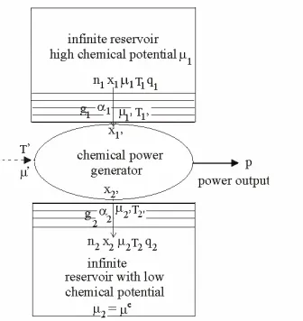
[image:3.612.100.268.344.522.2]III. CHEMICAL SYSTEMS WITH STEADY POWER OUTPUT Thermodynamic approaches can be applied to power optimization in chemical and electro-chemical engines. In chemical engines, Fig. 2, mass transports drive transformation of chemical energy into mechanical power. Yet, as opposed to thermal machines, in chemical ones generalized streams or reservoirs are present, capable of providing both heat and substance [6].
Figure 2. Scheme of a chemical engine controlled by a suitable choice of Carnot variables T’and µ’.
Large streams or infinite reservoirs assure constancy of chemical potentials. Problems of maximum of power produced or minimum of power consumed are then static problems. For a finite “upper reservoir”, however, the amount and chemical potential of an active reactant decrease in time, and considered problems are those of dynamic optimization and variational calculus. This motivates the use of the optimization algorithm presented in Sec. II.
Because of the diversity and complexity of chemical systems the area of power producing chemistries is broad. The simplest model of power producing chemical engine is that with an isothermal isomerization reaction, A1-A2=0 [5, 6]. Power expression and efficiency formula for the chemical system follow from the entropy conservation and energy balance in the power-producing zone of the system (‘active part’). In an ‘endoreversible chemical engine’ total entropy
flux is continuous through the active zone. When a formula describing this continuity is combined with energy balance we find in an isothermal case
p=(µ1'−µ2')n1, (17)
where n1=n is an invariant molar flux of reagents for the reactor with a complete conversion. Process efficiency ζ is defined as power yield per molar flux, n, i.e.
' 2 ' 1
/ µ µ
ζ =p n= − (18) This efficiency is identical with the chemical affinity of our reaction in the chemically active part of the system. While ζ is not dimensionless, it describes correctly the system.
In terms of Carnot control, µ’, [1], the efficiency is 2
− ′
=µ µ
ζ . (19) For a steady engine the following function describes Carnot control µ’ in terms of fuel flux n = n1 and its mole fraction x
1
1 1 1
2 0 1
1 2 2
ln x n g RT
n g x
µ µ ζ
− −
−
′ = + +
+
(20)
An associated formula defines the chemical efficiency in terms of flux n and mole fraction x. Its consequence is the sketch of flux n in terms of efficiency in Fig.3
+ − +
= −
−
2 1 2
1 1 1
0 ln
x ng
ng x RT ζ
ζ (21)
Figure 3. Fuel flux n in a chemical engine in terms of the efficiency of power production ζ.
Equation (21) shows that an effective concentration of the reactant in upper reservoir x1eff = x1 – g1-1n is decreased, whereas an effective concentration of the product in lower reservoir x2eff = x2 + g2-1n is increased due to the finite mass flux. Therefore, as shown in Fig.3, the fuel flux, n, decreases nonlinearly with the efficiency ζ. When the effect of resistances −1
k
g is ignorable, the reversible efficiency, ζC, can be attained, yet for finite resistances and efficiencies in the vicinity of ζC fuel flux n must be very small. Extensions of Eq. (21) are available for complex multireaction systems [12].
The power function, described by the product p=ζ(n)n, exhibits a maximum for a finite value of the fuel flux, n. The location of optimal n may be found from the graph of power
engine range n (ζ)
ζ ζC
[image:3.612.317.540.395.537.2]p=ζ(n)n. This “static” case of the optimization is described in details in the previous publications [1,5,6].
IV. OPTIMIZATION OF POWER IN DYNAMIC SYSTEMS For the reaction considered, a related dynamical problem may be formulated. It refers to a cascade of small engines in Fig.2. Application of Eq. (21) to an unsteady system leads to a work function describing the dynamical limit of the system
1 1 1 2 1 0 / / ) 1 /( ln 1 1 τ τ τ τ ζ τ τ d d dX d jdX x d dX X X RT W f i − + + + −
=
∫
(22)(X=x/(1-x).) Here X=x/(1-x) and j equals the ratio of upper to lower mass conductance, g1/g2 [6]. The path optimality condition may be expressed as the constancy condition for the following Hamiltonian + + = + = 2 2 2 1 1 2 2 1 ) ( ) ( ) , ( x j X X X RT x X x X jx x X RT X X
H & & & . (23)
For low rates and large concentrations X (mole fractions x1 close to the unity) optimal relaxation rate is approximately constant. Yet, in an arbitrary situation optimal rates are state dependent so as to preserve the constancy of H in Eq. (23).
The Hamiltonian H in Eq. (23) is of “energy type”, which means that it is an additive component of the enlarged Hamiltonian of Sec. 2. In the optimal process both Hamiltonians differ by a constant time adjoint zt,
opt n t n opt n
opt H z
H~ −1≡ −1 +( −1) (24) As zt is constant in optimal autonomous systems the maximization of each Hamiltonian with respect to controls leads to the same optimality conditions.
The analytical theory for the optimal criterion (22) leads to a partial differential equation usually called the Hamilton-Jacobi-Bellman equation (HJB equation [1,10])
0 = ∂ ∂ + − + + 1 + + ∂ ∂ − 2 1 − 0 1 1 u X V ju x u X X RT V u ) ( ln max ) ( ζ τ τ (25) where u=dX/dτ1
. As it is impossible to solve this equation analytically, we describe below numerical solving based on the Bellman’s method of dynamic programming (DP; [17]).
V. DISCRETE MODEL FOR NUMERICAL OPTIMIZATION Considering computer needs we introduce a related discrete scheme. In the discrete optimization context one has to search for the maximum of the performance index
k k k k k k N k N u ju x u X X RT
W ζ θ
− + + + − = − =
∑
2 1 1 1 0 1 ) 1 (ln
(26)
(j≡g1/g2) with the difference constraints
k k k k u X
X − −1=
θ
1
1 (27) k
k k
θ
τ
τ
− −1= (28)We search for maximum of the sum (26) subject to discrete constraints (27) and (28). In particular, the task includes the defining a solving algorithm for the discrete set in question and conditions when the numerical schemes of dynamic programming for the set (26)-(28) converge to solutions of the Hamilton-Jacobi-Bellman equation (25), [4].
While the analytical treatment of Eq. (25) is a quite difficult task, it is quite easy to solve numerically the related Bellman’s recurrence equation of dynamic programming (DP; [17]). Consequently, we apply the DP method to search for the solution of Bellman’s recurrence equation. In terms of cost function l0n ≡−f0na general form of this equation is
)}, , ) , , , ( (( ) , , , ( { min ) , ( , n n n n n n n n n n n n n n n n n n n t t R t l t R n n θ θ θ θ θ θ − − + = 1 − 0 u x f x u x x
u (29)
where Rn (xn, tn) = min (-Wn)is the function describing the problem in terms of the minimum of power consumed. This is a function of optimal cost type. In an isothermal case x=X1, u=u and t=τ1. Applying Eq. (29) to the problem described by
Eqs. (26) - (28), leads to the following recurrence equation
k k k k k k k k k θ u ju x u X X RT X R k k − + + + = − 2 1 1 1 0 ) 1 ( ln min ) , (
{
, ζ τ θ u}
) , (( 11 k n k k k
n
u
θ
X
R −
τ
−θ
+ − . (30) This is the discrete recurrence structure whose solution approximates for large number of stages the solution of the continuous HJB equation ( 27). Numerical solving of Eq. (30) is quite easy. Low dimensionality of the state vector in Eq. (30) assures a decent accuracy of DP solution. Moreover, an original accuracy can be significantly improved after performing the so-called dimensionality reduction associated with the elimination of time tn as the state variable. In the transformed problem, without coordinate tn, accuracy of DP solutions is high (see Chapters 7 and 9 of book [1]).
VI. ELECTROCHEMICAL ENGINES: FUEL CELLS Power maximization approaches can also be applied to electrochemical engines, in particular fuel cells [18, 19].
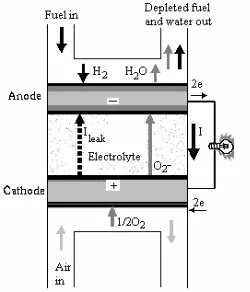
A fuel cell (Fig.4) is an electrochemical energy converter which directly and continuously transforms a part of chemical energy into electrical energy by consuming fuel and oxidant. Fuel cells have attracted great attention by virtue of their inherently clean and reliable performance. Their main advantage as compared to heat engines is that their efficiency is not a major function of device size.
Figure 4. Principle of a solid oxide fuel cell
Reversible cell voltage E0 is often a reference basis calculated from the Nernst equation. Yet, in more general cases, actual voltage without load must take into account losses of the idle run, which are the effect of flaws in electrode constructions and other imperfections.
In [19] the operating voltage of a cell is evaluated as the departure from the idle run voltage E0
V
=
E
0-
V
int=
E
0-
V
act-
V
conc-
V
ohm (31) Losses, which are called polarization, include three main sources: activation polarization (Vact), ohmic polarization (Vohm), and concentration polarization (Vconc). Activation and concentration polarization occurs at both anode and cathode locations, while the resistive losses occur throughout the cell.An example of the experimental data of voltage and power in a SOFC is shown in Fig. 5.
Figure 5. Voltage-current density and power-current density characteristics of the SOFC for various temperatures. Continuous lines represent the Aspen PlusTM calculations testing the model consistency with the experiments. These lines were obtained in Wierzbicki’s MsD thesis supervised by S. Sieniutycz and J. Jewulski [19]. Points refer to experiments of Wierzbicki and Jewulski in Warsaw Institute of Energetics ([19] and ref [18] therein).
Power density is the product of voltage V and current density i. Large number of approaches for calculating polarization losses has been presented in literature, as
reviewed in [18]. Both theory and experiments show power maxima in fuel cells [18,19]. As the voltage losses increase monotonically with current, the initially increasing power begins finally to decrease for sufficiently large currents, so that the emergence of power maxima is obvious [18, 19].
Power effects in thermal and electrochemical systems can be treated jointly (Sec. VII). Power data subsume effects of irreversible transports, reversible voltage and the detrimental effect of the idle run attributed to the electrode flaws.
VII. THEORETICAL POWER LIMITS IN ELECTROCHEMICAL GENERATORS
Theoretical evaluation of power limits in (electro)chemical generators and fuel cells is an important problem. Let us focus on fuel cells described by the formalism of inert components [20, 21] rather than the ionic description [22].
Assume, for simplicity, that the active (power producing) driving forces involve only: one temperature difference, single chemical affinity and an operating voltage φ1 - φ2. A generalization involving more affinities is obvious.
Total power production is the sum of thermal, substantial and electric components, i.e.
e n e s n s
e n s
I I R I I R I I R
I R I R I R
I I
I T T
I I
I T T P
ne se
sn
ee nn ss
e n
2 s
2 1
e 2' 1' n 2' 1' s 2' 1'
) ( ) ( ) -(
) ( ) (
) (
− −
−
− − −
− + − + =
− + −
+ − =
2 2 2
2 1 1 µ φ φ
µ
φ φ µ
µ
(32)
After introducing the enlarged vector of all driving potentials
µ
~= (T,µµµµ, V), the flux vector of all currents and the overall resistance tensor R~ , Eq. (32) can be written in a simple matrix-vector form
p=(µ~1−µ~2).~Ι− R~:~I~I . (33) Maximum power corresponds with the vanishing of the partial derivative vector
∂p/∂~Ι =µ~1−µ~2−2R~.~I =0. (34) Therefore, the optimal (power-maximizing) vector of currents at the maximum point of the system can be written in the form
~Imp R~ .(µ~ µ~2) ~IF
2 1 ≡ − 2
1
= −1 1 (35)
This result means that the power-maximizing current vector in strictly linear systems equals one half of the purely dissipative current at the Fourier-Onsager point, at which no power production occurs. Moreover, we note that Eqs. (33) and (35) yield the following result for the maximum power limit of the system
) ~ ~ .( ~ ). ~ ~ ( 4 1
2 1 1 2
1 µ R µ µ
µ − −
= −
mp
[image:5.612.68.302.438.598.2]In terms of the purely dissipative flux vector at the Fourier-Onsager point, the above limit of maximum power is represented by an equation
~:~ ~
4 1
F F mp
p = R I I (37)
Of course, the power dissipated at the Fourier-Onsager point equals
pF=R~:~IF~IF (38) Equations (37) and (38) prove that, in linear systems, only at most 25% of power (38), dissipated in the natural transfer process, can be transformed into the noble form of the mechanical power. This is a general result which, probably, cannot be easily generalized to nonlinear transfer systems where significant deviations from Eq. (37) could be possible depending on the nature of diverse nonlinearities. Despite of the limitation of the result (37) to linear transfer systems its value is significant because it shows explicitly the order of magnitude of thermodynamic limitations in power production systems. The above analysis also proves that a link exists between the mathematics of the thermal engines and fuel cells, and also that the theory of fuel cells can be unified with the theory of thermal and chemical power generators.
VIII. CONCLUSIONS
This research provides data for the power production limits which are enhanced in comparison with those predicted by the classical thermodynamics. Our power limits are “thermokinetic” rather than “thermostatic”. In fact, thermostatic limits are often too far from reality to be really useful. Generalized limits, obtained here, are more exact and informative than those predicted by the thermostatic theory. As opposed to the limits of classical thermodynamics, generalized limits depend not only on state changes of resources but also on process resistances, process direction and mechanism of heat and mass transfer.
Common methodology was developed for thermal, chemical and electrochemical systems. Fuel cells are included into this methodology. It is shown that, with irreversible thermodynamics, we can predict power limits for quite diverse practical systems.
The future of power production will certainly include fuel cell systems. The fuel cell operates continuously generating electricity as long as the fuel and oxidant are supplied. In fact, fuel cells have recently attracted great attention by virtue of their inherently clean, very efficient, and reliable performance. Major advantage of fuel cells compared to heat engines is that their efficiency is not a major function of device size. Fuel cells are particularly suitable when they are used in relatively small systems requiring very clean energy. In this paper effect of incomplete conversions in SOFC’s has been modeled by assuming that substrates can be remained after the reaction and that side reactions may occur. Optimum and feasibility conditions are discussed for basic input parameters of the cell. The developed FC model describes the performance of fuel cells at various operating conditions. Lowering of SOFC efficiency is linked with polarizations (activation, concentration and ohmic) and
incomplete conversions. Power limits for fuel cells are obtained in terms of parameters such as efficiency, resource input, and electric current density. Experiments confirm that the power data differ for power generated and consumed, and depend on system’s parameters, e.g., current intensity, number of mass transfer units, polarizations, electrode surface, average chemical rate, etc.. These data define bounds for SOFC energy generators, which are more informative than the familiar reversible bounds evaluated for electrochemical transformations.
REFERENCES
[1] S. Sieniutycz and J. Jeżowski, Energy Optimization in Process Systems, Chap.3, Elsevier, Oxford, 2009.
[2] S. Sieniutycz, “Carnot controls to unify traditional and work-assisted operations with heat & mass transfer”, International J. of Applied Thermodynamics, 6 (2003), 59-67.
[3] S. Sieniutycz, “Complex chemical systems with power production driven by mass transfer”, Intern. J. of Heat and Mass Transfer, 52 (2009), 2453-2465.
[4] S. Sieniutycz, “Dynamic programming and Lagrange multipliers for active relaxation of fluids in non-equilibrium systems”, Applied Mathematical Modeling, 33 (2009), 1457-1478.
[5] A. de Vos, Endoreversible Thermodynamics of Solar Energy Conversion, pp.30-41, Oxford University Press, Oxford, 1994. [6] S. Sieniutycz, “An analysis of power and entropy generation in a
chemical engine,” Intern. J. of Heat and Mass Transfer 51 (2008) 5859–5871.
[7] A. Poświata, Optimization of Drying Processes with Fine Solid in Buble Fluidized Bed, PhD thesis, Faculty of Chemical & Process Engineering, Warsaw Technological University Press, Warsaw 2005. [8] S. Sieniutycz, “State transformations and Hamiltonian structures for
optimal control in discrete systems”, Reports on Mathematical Physics 57 (2006), 289-317.
[9] S. Sieniutycz, “The constant Hamiltonian problem and an introduction to the mechanics of optimal discrete Systems”, Reports of Inst. of Chem. Eng. at Warsaw Tech. University, 3(1974), 27-53.
[10] S. Sieniutycz, Optimization in Process Engineering, 2-nd edn, Wydawnictwa Naukowo Techniczne, Warszawa, 1991.
[11] L. T. Fan and C.S. Wang, The Discrete Maximum Principle, A Study of Multistage System Optimization, Wiley, New York, 1964.
[12] H. Halkin, “A maximum principle of the Pontryagin type for systems described by nonlinear difference equations”, SIAM J. Control, ser. A, 4(1966), 528-547.
[13] M.D. Canon, C.D., Cullun and E.R. Polak, Theory of Optimal Control and Mathematical Programming, Wiley, New York, 1972. [14] V.G. Boltyanskii, Optimal Control of Discrete Systems, Nauka,
Moscow, 1973.
[15] S. Sieniutycz and R.S. Berry, “Discrete Hamiltonian analysis of endoreversible thermal cascades”, Chap. 6 (p. 143-172) in: S. Sieniutycz and A. de Vos, eds, Thermodynamics of Energy Conversion and Transport, Springer, New York, 2000.
[16] A. Poświata and Z. Szwast, “Optimization of fine solid drying in bubble fluidized bed”, Transport in Porous Media, 2 (2006), 785-792. [17] R. E. Bellman, Adaptive Control Processes: a Guided Tour,
Princeton, University Press, 1961, pp.1-35.
[18] Z. Zhao, C. Ou and J. Chen, “A new analytical approach to model and evaluate the performance of a class of irreversible fuel cells, International Journal of Hydrogen Energy, 33(2008), 4161- 4170. [19] M. Wierzbicki, Optimization of SOFC Based Energy System Using
Aspen PlusTM, MsD Thesis, The Faculty of Chemical and Process
Engineering, Warsaw University of Technology Press, Warsaw 2009. [20] B.R. Sundheim, “Transport properties of liquid electrolytes”, p.p.
165-254 in B.R. Sundheim, ed., Fused Salts, Mc Graw Hill, New York, 1964.
[21] A. Ekman, S. Liukkonen and K. Kontturi, “Diffusion and electric conduction in multicomponent electrolyte systems”, Electrochemica Acta, 23(1978), 243-250.