Combined beef thawing using response surface methodology

Beef is rich in nutrients and proteins, but low in fats and cholesterols, and thus is increasingly popularised among customers (Manios & Skandamis 2015). With the gradual development of the beef industry, freezing has become one of the most frequently used preservation methods for meat and meat products (Kovačević & Mastanjević 2011; Khaleque et al. 2016; Ngapo & Vachon 2016; Liu et al. 2016). The final edible quality of frozen meat is largely associated with the subsequent thawing method. However, the thawing process is faced with problems of juice loss, discoloration, and energy dissipation, so exploring new efficient and energy-saving thawing techniques is very meaningful.

Currently, the commonly used thawing methods for meat products in factories are air thawing and water thawing. Air thawing is limited by long time consumption, large occupied area, and poor colour. Water thawing is limited by large juice loss and mi-crobial contamination (Kim et al. 2015).

Beef rib-eye was treated by four thawing methods separately [still air thawing (SAT), still water thawing (SWT), ultrasonic thawing (UT), microwave thawing (MT)], and then investigated in terms of four indices [pH, drip loss rate (DLR), cooking loss rate (CLR), protein content (PC)]. On this basis, regression equa-tions were established via response surface methodol-ogy (RSM) and used to investigate the optimal beef thawing process. This study provides a theoretical basis for optimal combined thawing of beef rib-eye.

MATERIAL AND METHODS

Materials. Healthy Woking Black Cattle (Chang-chun Haoyue Islamic Meat Co. Ltd., Jilin Province, China) fattened for more than 6 months (Wang et al. 2015). After 24 h of fasting and 8 h of water fasting, the animals were slaughtered according to China Beef Quality Grading (NY/T676-2003) and then

Combined Beef Thawing Using Response

Surface Methodology

Jiahui JIN, Xiaodan WANG, Yunxiu HAN, Yaoxuan CAI, Yingming CAI, Hongmei WANG, Lingtao ZHU, Liping XU, Lei ZHAO and Zhiyuan LI

College of Food Science and Engineering, Jilin University, Changchun, P.R. China

Abstract

Jin J., Wang X., Han Y., Cai Y., Cai Y., Wang H., Zhu L., Xu L., Zhao L., Li Z. (2016): Combined beef thaw-ing usthaw-ing response surface methodology. Czech J. Food Sci., 34: 547–553.

Based on four thawing methods (still air, still water, ultrasonic wave, and microwave) and single-factor tests, we estab-lished a four-factor three-level response surface methodology for a regression model (four factors: pH, drip loss rate, cooking loss rate, protein content). The optimal combined thawing method for beef rib-eye is: microwave thawing (35 s work/10 s stop, totally 170 s) until beef surfaces soften, then air thawing at 15°C until the beef centre tempera-ture reaches –8°C, and finally ultrasonic thawing at 220 W until the beef centre temperatempera-ture rises to 0°C. With this method, the drip loss rate is 1.9003%, cooking loss rate is 33.3997%, and protein content is 229.603 μg, which are not significantly different from the model-predicted theoretical results (P ≥ 0.05).

Keywords: microwave; Box-Behnken; thaw; ultrasound

cooled for 24 h (Smékal et al. 2005). Rib-eye parts were randomly cut out from different animals and cut into cubes (80 × 80 × 20 mm). Totally 60 cubes (each 150.0 ± 2.0 g) were stored in a freezer. The temperature in the cube centre should be –18°C.

Thawing methods. A total of four kinds of thaw-ing methods: SAT, SWT, UT, and MT (Table 1). Each thawing method has 5 conditions, use the correspond-ing method of thawcorrespond-ing to each condition, which is a single and discontinuous thawing. The method is considered to be a single-factor experiment, and only once thawed at each condition. For example, thawing beef at 15°C, four parameters of pH, DLR, CLR, and PC were measured, data were recorded, and then beef was thawed at 20°C and four indicators were measured. Specifically, work time periods of MT were separated by 10 seconds. Namely, at condition No. 1, each time MT worked for 10 s and stopped for 10 s, until the temperature in a sample centre reached 0°C.

pH detection. pH was measured as defined by China Standard GB/T 9695.5:2008: 5 g of beef was ground and 45 ml of ultrapure water were added; then pH was measured with a pH meter 3 times and the average value was used.

DLR. Each sample was weighed on the FA1604 ana-lytical balance. Then DLR was computed as follows: DLR = (m₁ – m₂)/m₁ × 100% (1)

where: m₁ – weight before thawing (g); m₂ – weight after thawing (g)

Each experiment was measured 3 times and the average value was used.

CLR. Each sample was placed in a valve bag and put into a water bath at 80°C for 30 min, thawed under 20°C flowing water. Then the surface water was sucked off with absorbent paper and the sample was weighed (Xiong et al. 2012). CLR was computed as follows: CLR = (m₁– m₂)/m₁ × 100% (2)

where: m₁– weight after cooking (g); m₂– weight before cooking (g)

Each experiment was measured 3 times and the average value was used.

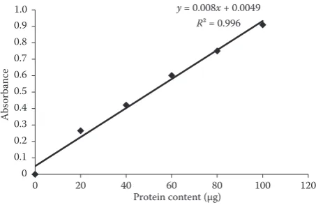
PC. First, 100 μg/ml bovine serum albumin (BSA) was prepared. Different amounts of BSA were add-ed with Coomassie brilliant blue G-250 to create a concentration gradient (Saeed et al. 2010). After standing for 5 min, these solutions were detected colorimetrically at 595 nm using a ZY053688 spec-trophotometer and the absorbance was recorded. A standard curve with PC as the x-axis and absorbance as the y-axis was plotted.

As shown in Figure 1, the equation is y = 0.008x + 0.049 (R2 _{= 0.996). Then the beef samples as treated}

were fully mixed with Coomassie G-250 and sent to detection of absorbance. Then PC was computed via the standard curve as follows:

PC (mg/g) = (C × VT)/(1000 VS × WF) (3)

where: C – value determined from the standard curve (µg); VT – total volume of the extract (ml); WF – fresh weight of a sample (g); VS – volume of added sample (ml)

Selection of RSM factors and levels. Based on single-factor experiments and the Box-Behnken de-sign of combination experiment (Cheng et al. 2014), we established a four-factor three-level RSM test. Each of the four factors (x₁, x₂, x₃, x₄) was assigned a low, medium, and high level, marked as –1, 0, 1, Table 1. Condition settings for different thawing methods

Thawing

methods Variable

Set conditions No.

1 2 3 4 5

SAT temperature (°C) 15 20 25 30 35

SWT temperature (°C) 2 10 20 30 40

UT power (W) 100 150 200 250 300

MT work time per interval (s) 10 20 30 40 50

SAT – still air thawing, SWT – still water thawing, UT – ultrasonic thawing, MT – microwave thawing

y= 0.008x+ 0.0049

R² = 0.996

0 0.1 0.2 0.3 0.4 0.5 0.6 0.7 0.8 0.9 1.0

0 20 40 60 80 100 120

A

bs

or

ba

nc

e

Protein content (μg)

respectively (Table 2). Four thawing methods were followed by thawing a piece of meat.

Statistical analysis. Statistical analyses and plot-ting were conducted by Excel 2007 and Design-Expert 8.0.6 software (Ghafoor et al. 2011). The analyses of variance were performed by the ANOVA proce-dure. The mean values were considered significantly different when P < 0.05.

RESULTS AND DISCUSSION

Single-factor analysis

Effects of thawing methods on beef pH. The pH of grade I, II, and III (degenerated) freshness is 5.8–6.2, 6.3–6.6, and > 6.7, respectively. As shown in Figure 2, as for SAT, pH increases at first and then it drops. As for SWT and UT, pH declines at first and then it increases. The reason is that due to the interruption of oxygen supply after slaughter, muscle glycogen undergoes anaerobic glycolysis, so under the action of a glycolytic enzyme pH drops. With the increase of water temperature or ultrasonic power, a part of the enzyme is inactivated, leading to the termination of an acid- producing reaction. As for MT, pH rises because the microwaves could affect the components of muscle ions. The pH values differ after different

thawing treatments, but they are generally within the normal range, indicating good quality.

Effects of thawing methods on DLR. The thaw-ing treatment would induce the drip loss of abun-dant soluble proteins, leading to the loss of nutrients (Šimoniová et al. 2013). As shown in Figure 3A, as for SAT, the DLR increases because a lower air temperature is less likely to change water density and thereby less able to promote water migration. As for SWT (UT), the DLR declines at first and then it rises. Because ultrasonic waves alter the structure of original beef tissues, a further increment of acoustic wave destroys the cell structure, causing the juice loss. As for MT, the DLR declines at first and then it rises. The rea-son is that a too short work time would prolong the thawing time; a too long work time would promote the absorption of microwaves, so the uneven heating makes the thawing effect unfavourable.

Effects of thawing methods on CLR. During the freezing process, the ice crystals would destroy the meat tissues, leading to a significant change in cook-ing loss (Muela et al. 2015). As shown in Figure 3B, as for SAT, the CLR increases. A possible reason is that meat freezing would destroy cell membranes, while the muscle cellular water holding capacity is Table 2. Independent variables and their levels in the

response surface design

Factors (levels) –1 0 1

x₁ SAT (°C) 10 15 20

x₂ SWT (°C) 15 20 25

x₃ UT (W) 150 200 250

x₄ MT (s) 20 30 40

Figure 2. The pH value of beef rib-eye muscle after dif-ferent thawing methods

SAT – still air thawing, SWT – still water thawing, UT – ul-trasonic thawing, MT – microwave thawing

5.80 5.85 5.90 5.95 6.00 6.05 6.10 6.15

1 2 3 4 5

pH

Set number

SAT SWT

UT MT

Figure 3. The drip loss (A) and cooking loss (B) of beef rib-eye muscle after different thawing methods

SAT – still air thawing, SWT – still water thawing, UT – ul-trasonic thawing, MT – microwave thawing

1.0 1.5 2.0 2.5 3.0 3.5 4.0 4.5 5.0 5.5

1 2 3 4 5

Drip loss rate (%)

Set number

SAT SWT

UT MT

33 34 35 36 37 38 39 40 41 42

1 2 3 4 5

Cooking loss rate (%)

Set number

SAT SWT

UT MT

(A)

reserved at a low temperature, which prevents the cooking loss. CLR drops at first and then it rises with the increase of water temperature (SWT), power (UT), or work time per segment (MT).

Effects of thawing methods on beef PC. As shown in Figure 4, as for SAT, PC gradually declines because the rise of air temperature promotes the oxidation of beef proteins to form carbonyl and disulphide bonds, thus changing the conformation of proteins. As for SWT, PC increases at first and then it declines, probably because a too low water temperature would prolong the thawing time and cause the loss of water-soluble proteins; a too high water temperature would cause cross-linking, degradation, and degeneration of actin. As for UT, PC rises at first and then it declines. The reason is that too small power leads to a prolonged

thawing time, so the molecular forces that maintain the integrity of muscle tissues are destroyed while too large power would promote the contraction of mus-Figure 4. Protein content of beef rib-eye muscle after dif-ferent thawing methods

SAT – still air thawing, SWT – still water thawing, UT – ul-trasonic thawing, MT – microwave thawing

220 222 224 226 228 230

1 2 3 4 5

Protein content (μg)

Set number

SAT SWT

UT MT

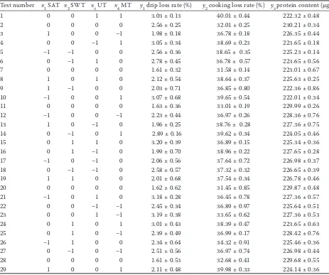
Table 3. Response surface methodology

Test number x₁ SAT x₂ SWT x₃ UT x₄ MT y₁ drip loss rate (%) y₂ cooking loss rate (%) y₃ protein content (μg)

1 0 0 1 1  3.03 ± 0.13 40.01 ± 0.44 222.32 ± 0.48

2 0 0 0 0 2.56 ± 0.25 32.01 ± 0.25 230.21 ± 0.34

3 1 0 0 –1 1.98 ± 0.18 36.78 ± 0.18 226.35 ± 0.44

4 0 0 –1 1 3.05 ± 0.34 38.69 ± 0.23 223.65 ± 0.18

5 –1 –1 0 0 2.56 ± 0.36 38.65 ± 0.35 225.23 ± 0.14

6 0 –1 1 0 2.78 ± 0.45 36.78 ± 0.57 223.65 ± 0.56

7 0 0 0 0 1.61 ± 0.32 31.58 ± 0.14 223.01 ± 0.67

8 1 0 1 0 2.12 ± 0.54 38.64 ± 0.37 225.63 ± 0.25

9 1 –1 0 0 2.03 ± 0.71 36.85 ± 0.80 222.36 ± 0.86

10 –1 0 0 1 3.07 ± 0.68 39.65 ± 0.54 222.01 ± 0.34

11 0 0 0 0 1.63 ± 0.36 33.01 ± 0.19 229.99 ± 0.26

12 –1 0 0 –1 2.23 ± 0.44 36.97 ± 0.26 228.36 ± 0.76

13 1 0 –1 0 1.96 ± 0.25 38.76 ± 0.28 227.36 ± 0.75

14 0 –1 0 1 2.89 ± 0.16 39.62 ± 0.34 224.05 ± 0.46

15 0 1 1 0 3.20 ± 0.39 36.89 ± 0.15 225.34 ± 0.36

16 0 1 –1 0 1.99 ± 0.70 38.96 ± 0.22 227.65 ± 0.28

17 –1 0 –1 0 2.06 ± 0.56 37.64 ± 0.72 226.98 ± 0.37

18 0 –1 –1 0 2.58 ± 0.57 37.32 ± 0.32 226.65 ± 0.39

19 1 1 0 0 2.01 ± 0.68 37.54 ± 0.34 226.78 ± 0.46

20 0 0 0 0 1.62 ± 0.62 31.45 ± 0.85 229.87 ± 0.48

21 –1 0 1 0 3.18 ± 0.28 36.45 ± 0.78 227.36 ± 0.57

22 0 0 –1 –1 2.45 ± 0.34 36.89 ± 0.97 225.64 ± 0.51

23 0 0 1 –1 3.19 ± 0.38 33.65 ± 0.62 227.36 ± 0.53

24 0 1 0 1 3.01 ± 0.43 38.39 ± 0.47 223.65 ± 0.63

25 0 1 0 –1 2.39 ± 0.49 36.99 ± 0.17 228.42 ± 0.76

26 –1 1 0 0 2.34 ± 0.64 34.32 ± 0.91 225.46 ± 0.36

27 0 –1 0 –1 2.51 ± 0.56 36.97 ± 0.74 226.98 ± 0.44

28 0 0 0 0 1.61 ± 0.53 32.68 ± 0.41 229.68 ± 0.55

29 1 0 0 1 2.11 ± 0.48 39.98 ± 0.33 224.14 ± 0.36

cle fibres, thus improving the protein degeneration (Stangierski et al. 2013). As for MT, PC increases at first and then it drops because a too short work time would improve the protein unfolding while a too long work time would excessively heat the meat surfaces and reduce the solubility of post-freezing proteins, manifested as a reduction of protein extractability.

RSM tests

RSM test arrangement and results. The beef pH levels were all within the normal range after each thawing treatment, so pH was not considered in the subsequent tests, and DLR (y₁), CLR (y₂), and PC (y₃) as response values, we designed and conducted 29 tests (24 factorial tests, 5 central tests) to estimate errors. The test scheme and results are listed in Table 3.

The regression equations underlying the effects of the four factors on y₁ are expressed as follows: y₁ = 1.81 – 0.27x₁ – 0.034x₂ + 0.28x₃ + 0.20x₄ + 0.050x₁x₂ – – 0.24x₁x₃ – 0.18x₁x₄ + 0.25x₂x₃ + 0.060x₂x₄ – – 0.19x₃x₄ + 0.023x₁2 _{+ 0.35x}

22+ 0.52x32+ 0.56x42 (4) The regression coefficients were sent to a signifi-cance test (Table 4).

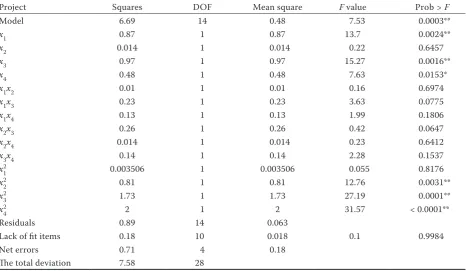
Table 4. The analysis of variance

Project Squares DOF Mean square F value Prob > F

Model 6.69 14 0.48 7.53 0.0003**

x₁ 0.87 1 0.87 13.7 0.0024**

x₂ 0.014 1 0.014 0.22 0.6457

x₃ 0.97 1 0.97 15.27 0.0016**

x₄ 0.48 1 0.48 7.63 0.0153*

x₁x₂ 0.01 1 0.01 0.16 0.6974

x₁x₃ 0.23 1 0.23 3.63 0.0775

x₁x₄ 0.13 1 0.13 1.99 0.1806

x₂x₃ 0.26 1 0.26 0.42 0.0647

x₂x₄ 0.014 1 0.014 0.23 0.6412

x₃x₄ 0.14 1 0.14 2.28 0.1537

x₁2 _{0.003506 1 0.003506 0.055 0.8176}

x₂2 _{0.81 1 0.81 12.76 0.0031**}

x₃2 _{1.73 1 1.73 27.19 0.0001**}

x₄2 _{2 1 2 31.57 < 0.0001**}

Residuals 0.89 14 0.063

Lack of fit items 0.18 10 0.018 0.1 0.9984

Net errors 0.71 4 0.18

The total deviation 7.58 28      

*P < 0.01 (extremely significant), **P < 0.05 (significant), P > 0.05 (non significant)

As shown in Table 4, the model item in the analy-sis of variance has ‘Pr > F’ = 0.0003, indicating this quadratic equation is extremely significant; the lack of fit has ‘Prob > F’ = 0.9984, indicating the equation fits well the tests and can be used to describe the real relationship between all factors and response value and thus to determine the optimal process conditions. Moreover, the linear terms x₁, x₃, and quadratic terms x₂2_{, x}

32, x42 are all very significant

(P < 0.01), the quadratic term x₄ is significant (P < 0.05), while the interaction items are not significant (P > 0.05). Thus, the effects of these factors on the response values are not simply linear. According to the coefficients, the effects of these factors on DLR change are as follows: UT > SWT > MT > SAT. The insignificant items at α = 0.05 were excluded, and the optimised regression equation is:

y₁ = 1.81 – 0.27x₁ + 0.28x₃ + 0.20 x₄ + 0.35x₂2_{+ 0.52x} 3 2₊ + 0.56x₄2 ₍₅₎

The regression coefficients of y₂ and y₃ were sent to significance tests, showing the two equations both fitted the tests well, and the optimised regression equation is:

y₂ = 32.15 – 1.51x₄ – 1.14x₃x₄ + 2.81x₁2 _{+ 2.45x} 2 2 ₊ + 2.62x₃2 _{+ 3.11x}

4

y₃ = 230.15 + 0.70x₂ + 1.94x₄ – 2.13x₁2 _{– 2.36x} 2 2 _{– 1.93x}

3 2 _–

– 2.77x₄2 _（7）

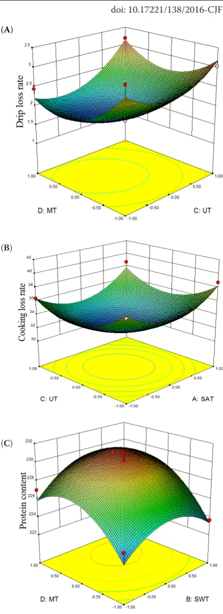
RSM analysis. RSM plots can well reflect the opti-mal parameters and the interaction among the param-eters (Herceget al. 2012). One image was selected for each of the three indices. At UT power = 200 W, DLR declines at first and then it increases with the prolonging of work time per segment during MT treatment (Figure 5A). Both UT and SAT achieve the minimum CLR at a zero level and each has an optimal point (Figure 5B). When MT is constant, with the rise of SWT temperature, PC increases at first and then it drops, and the response surface slope is very sharp, indicating PC is very sensitive to the MT-SWT interaction (Figure 5C).

Optimisation of extraction conditions. When the above regression model is used to predict the theoretically optimal response value, the extraction conditions are: x₁ = 0.457, x₂ = 0.421, x₃ = 0.282, x₄ = 0.489, namely SAT at 17.285°C, SWT at 22.105°C, UT at 214.1 W, and MT at 34.89 s, the juice loss rate is 1.95442%, the cooking loss is 33.4327%, the protein content is 229.584 μg. Given the real operational con-ditions, the optimal beef rib-eye extraction conditions are SAT temperature 15°C, SWT temperature 20°C, UT power 220 W, and MT work time 35 seconds.

Combination order under optimal thawing con-ditions. The ice, soon after melting to water, would absorb abundant microwave and thus cause local overheating and even aging (Lyng et al. 2013), so we selected MT as the first step. Results show neither SAT nor SWT would largely affect the subsequent thawing. From the perspective of industrial water saving, we replaced SWT by SAT. Ultrasonic waves function like mechanical waves and penetrate very strongly, so they were selected as the last step. These analyses were confirmed by the subsequent arranged combination tests, so the optimal combination is:

Figure 5. Response surface plots for effects of (A) mi-crowave thawing (MT) and ultrasonic thawing (UT) on drip loss rate (DLR), (B) UT and still air thawing (SAT) on cooking loss rate (CLR), and (C) MT and still water thawing (SWT) on Protein content (PC)

(A)

(B)

(C)

MT works for 35 s

and stops 10 s Surfaces of frozen beef softened

UT power 220 W SAT temperature

15°C Central temperature of frozen beef –8°C

Central temperature of beef 0°C

→

→

→

CONCLUSIONS

A quadratic regression model underlying relations between thawing methods (SAT, SW, TU, MT) and response values (DLR, CLR, PC) was established from the Design-Expert software.

The optimal beef thawing conditions are: MT (35 s operation/10 s stop, totally 170 s) until beef surfaces softened; SAT at 15°C until the beef centre tempera-ture reaches –8°C; UT at 220 W until the beef centre temperature rises 0°C. Under these conditions, the theoretical results are not significantly different from the verification results: DLR = 1.95442 vs. 1.9003%, CLR = 33.4327 vs. 33.3997%, and PC = 229.584 vs. 229.603 μg. Compared with the existing thawing methods used in factories, this new combined thawing method is manoeuvrable with higher thawed quality, higher price, and smaller input-output ratio. Thus, this method can be applied to reprocess thawed meat and frozen meat in factories.

References

Cheng A.W., Yan H.Q., Han C.J., Chen X.Y., Wang W.L., Xie C.Y., Qu J.R., Gong Z.Q., Shi X.Q. (2014): Acid and alka-line hydrolysis extraction of non-extractable polyphenols in blueberries: optimisation by response surface meth-odology. Czech Journal of Food Sciences, 32: 218–225. Ghafoor K., Hui T., Choi Y.H. (2011): Optimization of

ultrasonic-assisted extraction of total anthocyanins from grape peel using response surface methodology. Journal of Food Biochemistry, 35: 735–746.

Herceg Z., Juraga E., Sobota-Šalamon B., Režek-Jambrak A. (2012): Inactivation of mesophilic bacteria in milk by means of high intensity ultrasound using response surface methodology. Czech Journal of Food Sciences, 30: 108–117.

Khaleque M.A., Keya C.A., Hasan K.N., Hoque M.M., Inatsu Y., Bari M.L. (2016): Use of cloves and cinnamon essential oil to inactivate Listeria monocytogenes in ground beef at freezing and refrigeration temperatures. Food Science and Technology, 74: 219–223.

Kim Y.H., Liesse C., Kemp R., Balan P. (2015): Evaluation of combined effects of ageing period and freezing rate on quality attributes of beef loins. Meat Science, 110: 40–45.

Corresponding author:

Dr Xiao Dan Wang, Jilin University, College of Food Science and Engineering, Changchun 130062, P.R. China; E-mail: jxd@jlu.edu.cn

Kovačević D., Mastanjević K. (2011): Cryoprotective effect of trehalose and maltose on washed and frozen stored beef meat. Czech Journal of Food Sciences, 29: 15–23. Liu Y.Q., Mao Y.W., Liang R.R., Zhang Y.M., Wang R.H.,

Zhu L.X., Han G.X., Luo X. (2016): Effect of suspension method on meat quality and ultra-structure of Chinese Yellow Cattle under 12–18°C pre-rigor temperature con-trolled chilling. Meat Science, 115: 45–49.

Lyng J.G., Zhang L., Marra F., Brunton N.P. (2013): Effect of freezing rate and comminution on dielectric properties of pork. Czech Journal of Food Sciences, 31: 413–418. Manios S.G., Skandamis P.N. (2015): Effect of frozen

stor-age, different thawing methods and cooking processes on the survival of Salmonella spp. and Escherichia coli

O157:H7 in commercially shaped beef patties. Meat Sci-ence, 101: 25–32.

Muela E., Monge P., Sañudo C., Campo M.M., Beltrán J.A. (2015): Meat quality of lamb frozen stored up to 21 months: Instrumental analyses on thawed meat during display. Meat Science, 102: 35–40.

Ngapo T.M., Vachon L. (2016): Umami and related com-ponents in ‘chilled’ pork for the Japanese market. Meat Science, 121: 365–374.

Saeed S.M., Abdullah S.U., Sayeed S.A., Ali R. (2010): Food protein: food colour interactions and its application in rapid protein assay. Czech Journal of Food Sciences, 28: 506–513. Šimoniová A., Rohlík B., Škorpilová T., Petrová M., Pipek P. (2013): Differentiation between fresh and thawed chicken meats. Czech Journal of Food Sciences, 31: 108–115. Smékal O., Pipek P., Miyara M., Jeleníková J. (2005): Use of

video image analysis for the evaluation of beef carcasses. Czech Journal of Food Sciences, 23: 240–245.

Stangierski J., Rezler R., Baranowska H.M., Poliszko S. (2013): Effect of enzymatic modification on frozen chick-en surimi. Czech Journal of Food Scichick-ences, 31: 203–210. Wang X.D., Sun Y.H., Liu A.Y., Wang X.M., Gao J., Fan

X.C., Shang J.Y., Wang Y. (2015): Modeling structural and compositional changes of beef during human chewing process. Food Science and Technology, 60: 1219–1225. Xiong G.Y., Zhang L.L., Zhang W., Wu J. (2012): Influence of

ultrasound and proteolytic enzyme inhibitors on muscle degradation, tenderness, and cooking loss of hens dur-ing agdur-ing. Czech Journal of Food Sciences, 30: 195–205.