DOC: Deep Open Classification of Text Documents
Lei Shu, Hu Xu, Bing Liu Department of Computer Science
University of Illinois at Chicago
{lshu3, hxu48, liub}@uic.edu
Abstract
Traditional supervised learning makes the closed-world assumption that the classes appeared in the test data must have ap-peared in training. This also applies to text learning or text classification. As learning is used increasingly in dynamic open envi-ronments where some new/test documents may not belong to any of the training classes, identifying these novel documents during classification presents an important problem. This problem is called open-world classificationoropen classification. This paper proposes a novel deep learning based approach. It outperforms existing state-of-the-art techniques dramatically. 1 Introduction
A key assumption made by classic supervised text classification (or learning) is that classes appeared in the test data must have appeared in training, called theclosed-worldassumption (Fei and Liu, 2016; Chen and Liu, 2016). Although this as-sumption holds in many applications, it is violated in many others, especially in dynamic or open en-vironments. For example, in social media, a classi-fier built with past topics or classes may not be ef-fective in classifying future data because new top-ics appear constantly in social media (Fei et al., 2016). This is clearly true in other domains too, e.g., self-driving cars, where new objects may ap-pear in the scene all the time.
Ideally, in the text domain, the classifier should classify incoming documents to the right existing classes used in training and also detect those doc-uments that don’t belong to any of the existing classes. This problem is calledopen world classi-ficationoropen classification(Fei and Liu,2016). Such a classifier is aware what it does and does
not know. This paper proposes a novel technique to solve this problem.
Problem Definition: Given the training data
D = {(x1, y1),(x2, y2), . . . ,(xn, yn)}, wherexi
is thei-th document, and yi ∈ {l1, l2, . . . , lm} =
Y is xi’s class label, we want to build a model
f(x)that can classify each test instancexto one of themtraining orseenclasses inYor reject it to in-dicate that it does not belong to any of them train-ing or seen classes, i.e., unseen. In other words, we want to build a(m+ 1)-class classifierf(x) with the classesC={l1, l2, . . . , lm,rejection}.
There are some prior approaches for open clas-sification. One-class SVM (Sch¨olkopf et al.,2001; Tax and Duin, 2004) is the earliest approach. However, as no negative training data is used, one-class one-classifiers work poorly. Fei and Liu (2016) proposed a Center-Based Similarity (CBS) space learning method (Fei and Liu,2015). This method first computes a center for each class and trans-forms each document to a vector of similarities to the center. A binary classifier is then built us-ing the transformed data for each class. The deci-sion surface is like a “ball” encircling each class. Everything outside the ball is considered not be-longing to the class. Our proposed method outper-forms this method greatly.Fei et al.(2016) further added the capability of incrementally or cumula-tively learning new classes, which connects this work tolifelong learning(Chen and Liu,2016) be-cause without the ability to identify novel or new things and learn them, a system will never be able to learn by itself continually.
In computer vision,Scheirer et al.(2013) stud-ied the problem of recognizing unseen images that the system was not trained for by reducing open space risk. The basic idea is that a classifier should not cover too much open space where there are few or no training data. They proposed to re-duce the half-space of a binary SVM classifier
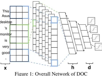
Figure 1: Overall Network of DOC with a positive region bounded by two parallel hyperplanes. Similar works were also done in a probability setting by Scheirer et al. (2014) and Jain et al.(2014). Both approaches use probabil-ity threshold, but choosing thresholds need prior knowledge, which is a weakness of the methods. Dalvi et al. (2013) proposed a multi-class semi-supervised method based on the EM algorithm. It has been shown that these methods are poorer than the method in (Fei and Liu,2016).
The work closest to ours is that in (Bendale and Boult,2016), which leverages an algorithm called OpenMax to add the rejection capability by uti-lizing the logits that are trained via closed-world softmax function. One weak assumption of Open-Max is that examples with equally likely logits are more likely from the unseen or rejection class, which can be examples that are hard to classify. Another weakness is that it requires validation ex-amples from the unseen/rejection class to tune the hyperparameters. Our method doesn’t make these weak assumptions and performs markedly better.
Our proposed method, called DOC (Deep Open Classification), uses deep learning (Goodfellow et al.,2016;Kim,2014). Unlike traditional clas-sifiers, DOC builds a multi-class classifier with a 1-vs-rest final layer of sigmoids rather than soft-max to reduce the open space risk. It reduces the open space risk further for rejection by tightening the decision boundaries of sigmoid functions with Gaussian fitting. Experimental results show that DOC dramatically outperforms state-of-the-art ex-isting approaches from both text classification and image classification domains.
2 The Proposed DOC Architecture DOC uses CNN (Collobert et al., 2011; Kim, 2014) as its base and augments it with a 1-vs-rest final sigmoid layer and Gaussian fitting for
classification. Note: other existing deep mod-els like RNN (Williams and Zipser,1989; Schus-ter and Paliwal,1997) and LSTM (Hochreiter and Schmidhuber, 1997; Gers et al., 2002) can also be adopted as the base. Similar to RNN, CNN also works on embedded sequential data (using 1D convolution on text instead of 2D convolution on images). We choose CNN because OpenMax uses CNN and CNN performs well on text (Kim,2014), which enables a fairer comparison with OpenMax.
2.1 CNN and Feed Forward Layers of DOC The proposed DOC system (given in Fig.1) is a variant of the CNN architecture (Collobert et al., 2011) for text classification (Kim, 2014)1. The first layer embeds words in documentxinto dense vectors. The second layer performs convolution over dense vectors using different filters of var-ied sizes (see Sec. 3.4). Next, the max-over-time pooling layer selects the maximum values from the results of the convolution layer to form a k -dimension feature vectorh. Then we reducehto am-dimension vectord=d1:m(mis the number
of training/seen classes) via 2 fully connected lay-ers and one intermediate ReLU activation layer:
d=W0(ReLU(W h+b)) +b0, (1)
where W ∈ Rr×k, b ∈ Rr, W0 ∈ Rm×r, and
b0 ∈ Rm are trainable weights; r is the output
dimension of the first fully connected layer. The output layer of DOC is a 1-vs-rest layer applied to
d1:m, which allows rejection. We describe it next.
2.2 1-vs-Rest Layer of DOC
Traditional multi-class classifiers (Goodfellow et al., 2016; Bendale and Boult, 2016) typically use softmax as the final output layer, which does not have the rejection capability since the prob-ability of prediction for each class is normalized across all training/seen classes. Instead, we build a 1-vs-rest layer containingm sigmoid functions formseen classes. For thei-th sigmoid function corresponding to classli, DOC takes all examples
withy = li as positive examples and all the rest
examplesy6=lias negative examples.
The model is trained with the objective of sum-mation of all log loss of themsigmoid functions
1https://github.com/alexander-rakhlin/
on the training dataD.
Loss=Xm
i=1
n
X
j=1
−I(yj =li) logp(yj =li)
−I(yj 6=li) log(1−p(yj =li)),
(2)
where I is the indicator function and p(yj =
li) =Sigmoid(dj,i)is the probability output from
ith sigmoid function on the jth document’s i th-dimension ofd.
During testing, we reinterpret the prediction of
msigmoid functions to allow rejection, as shown in Eq.3. For thei-th sigmoid function, we check if the predicted probability Sigmoid(di)is less than
a threshold ti belonging to class li. If all
pre-dicted probabilities are less than their correspond-ing thresholds for an example, the example is re-jected; otherwise, its predicted class is the one with the highest probability. Formally, we have
ˆ y=
reject, if Sigmoid(di)< ti,∀li∈ Y; arg maxli∈YSigmoid(di), otherwise.
(3)
Note that although multi-label classification (Huang et al., 2013; Zhang and Zhou, 2006; Tsoumakas and Katakis,2006) may also leverage multiple sigmoid functions, Eq. 3forbids multi-ple predicted labels for the same exammulti-ple, which is allowed in multi-label classification. DOC is also related to multi-task learning (Huang et al., 2013;Caruana, 1998), where each labelli is
re-lated to a 1-vs-rest binary classification task with shared representations from CNN and fully con-nected layers. However, Eq. 3performs classifi-cation and rejection based on the outputs of these binary classification tasks.
Comparison with OpenMax: OpenMax builds on the traditional closed-world multi-class classi-fier (softmax layer). It reduces the open space for each seen class, which is weak for rejecting unseen classes. DOC’s 1-vs-rest sigmoid layer provides a reasonable representation of all other classes (the rest of seen classes and unseen classes), and en-ables the 1 class forms a good boundary. Sec. 3.5 shows that this basic DOC is already much better than OpenMax. Below, we improve DOC further by tightening the decision boundaries more.
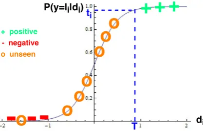
[image:3.595.311.520.68.202.2]2.3 Reducing Open Space Risk Further Sigmoid function usually uses the default prob-ability threshold of ti = 0.5 for classification of
Figure 2: Open space risk of sigmoid function and desired decision boundarydi=T and probability
thresholdti.
each class i. But this threshold does not con-sider potential open space risks from unseen (re-jection) class data. We can improve the bound-ary by increasing ti. We use Fig.2 to illustrate.
The x-axis representsdiand y-axis is the predicted
probability p(y = li|di). The sigmoid function
tries to push positive examples (belonging to the
i-th class) and negative examples (belonging to the other seen classes) away from the y-axis via a high gain arounddi= 0, which serves as the
de-fault decision boundary fordi withti = 0.5. As
demonstrated by those 3 circles on the right-hand side of the y-axis, during testing, unseen class ex-amples (circles) can easily fill in the gap between the y-axis and those dense positive (+) examples, which may reduce the recall of rejection and the precision of thei-th seen class prediction. Obvi-ously, a better decision boundary is at di = T,
where the decision boundary more closely “wrap” those dense positive examples with the probability thresholdti0.5.
To obtain a bettertifor each seen classi-th, we
use the idea of outlier detection in statistics:
1. Assume the predicted probabilities p(y =
li|xj, yj = li) of all training data of each
classi follow one half of the Gaussian dis-tribution (with meanµi = 1), e.g., the three
positive points in Fig. 2 projected to the y-axis (we don’t need di). We then
artifi-cially create the other half of the Gaussian distributed points (≥ 1): for each existing pointp(y =li|xj, yj =li), we create a
mir-ror point1 + (1−p(y=li|xj, yj =li)(not
a probability) mirrored on the mean of 1.
2. Estimate the standard deviationσiusing both
3. In statistics, if a value/point is a certain num-ber (α) of standard deviations away from the mean, it is considered an outlier. We thus set the probability thresholdti = max(0.5,1−
ασi). The commonly used number forαis 3,
which also works well in our experiments.
Note that due to Gaussian fitting, different class
lican have a different classification thresholdti.
3 Experimental Evaluation 3.1 Datasets
We perform evaluation using two publicly avail-able datasets, which are exactly the same datasets used in (Fei and Liu,2016).
(1) 20 Newsgroups2 (Rennie, 2008): The 20 newsgroups data set contains 20 non-overlapping classes. Each class has about 1000 documents.
(2)50-class reviews(Chen and Liu,2014): The dataset has Amazon reviews of 50 classes of ucts. Each class has 1000 reviews. Although prod-uct reviews are used, we do not do sentiment clas-sification. We still perform topic-based classifica-tion. That is, given a review, the system decides what class of product the review is about.
For every dataset, we keep a 20000 frequent word vocabulary. Each document is fixed to 2000-word length (cutting or padding when necessary). 3.2 Test Settings and Evaluation Metrics For a fair comparison, we use exactly the same set-tings as in (Fei and Liu,2016). For each class in each dataset, we randomly sampled 60% of docu-ments for training, 10% for validation and 30% for testing. Fei and Liu (2016) did not use a valida-tion set, but the test data is the same 30%. We use the validation set to avoid overfitting. For open-world evaluation, we hold out some classes (as un-seen) in training and mix them back during testing. We vary the number of training classes and use 25%, 50%, 75%, or 100% classes for training and all classes for testing. Here using 100% classes for training is the same as the traditional closed-world classification. Taking 20 newsgroups as an example, for 25% classes, we use 5 classes (we randomly choose 5 classes from 20 classes for 10 times and average the results, as in (Fei and Liu, 2016)) for training and all 20 classes for testing (15 classes are unseen in training). We use macro
F1-score over5 + 1 classes (1 for rejection) for
2http://qwone.com/˜jason/20Newsgroups/
Table 1: Macro-F1scores for 20 newsgroups % of seen classes 25% 50% 75% 100%
cbsSVM 59.3 70.1 72.0 85.2 OpenMax 35.7 59.9 76.2 91.9 DOC (t= 0.5) 75.9 84.0 87.4 92.6 DOC 82.3 85.2 86.2 92.6
Table 2: Macro-F1 scores for 50-class reviews % of seen classes 25% 50% 75% 100%
cbsSVM 55.7 61.5 58.6 63.4 OpenMax 41.6 57.0 64.2 69.2 DOC (t= 0.5) 51.1 63.6 66.2 69.8 DOC 61.2 64.8 66.6 69.8
evaluation. Please note that examples from unseen classes are dropped in the validation set.
3.3 Baselines
We compare DOC with two state-of-the-art meth-ods published in 2016 and one DOC variant.
cbsSVM: This is the latest method published in NLP (Fei and Liu, 2016). It uses SVM to build 1-vs-rest CBS classifiers for multiclass text classi-fication with rejection option. The results of this system are taken from (Fei and Liu,2016).
OpenMax: This is the latest method from com-puter vision (Bendale and Boult, 2016). Since it is a CNN-based method for image classification, we adapt it for text classification by using CNN with a softmax output layer, and adopt the Open-Max layer3for open text classification. When all classes are seen (100%), the result from softmax is reported since OpenMax layer always performs rejection. We use default hyperparameter values of OpenMax (Weibull tail size is set to 20).
DOC(t = 0.5): This is the basic DOC (t = 0.5). Gaussian fitting isn’t used to choose eachti.
Note that (Fei and Liu, 2016) compared with several other baselines. We don’t compare with them as it was shown that cbsSVM was superior.
3.4 Hyperparameter Setting
We use word vectors pre-trained from Google News4(3 million words and 300 dimensions). For the CNN layers, 3 filter sizes are used[3,4,5]. For each filter size, 150 filters are applied. The dimen-sionrof the first fully connected layer is 250.
3https://github.com/abhijitbendale/
OSDN
4https://code.google.com/archive/p/
3.5 Result Analysis
The results of 20 newsgroups and 50-class reviews are given in Tables1and2, respectively. From the tables, we can make the following observations:
1. DOC is markedly better than OpenMax and cbsSVM in macro-F1scores for both datasets in the 25%, 50%, and 75% settings. For the 25% and 50% settings (most test examples are from unseen classes), DOC is dramati-cally better. Even for 100% of traditional closed-world classification, it is consistently better too. DOC(t= 0.5) is better too. 2. For the 25% and 50% settings, DOC is also
markedly better than DOC(t = 0.5), which shows that Gaussian fitting finds a better probability threshold than t = 0.5 when many unseen classes are present. In the 75% setting (most test examples are from seen classes), DOC(t = 0.5) is slightly better for 20 newsgroups but worse for 50-class re-views. DOC sacrifices some recall of seen class examples for better precision, whilet= 0.5sacrifices the precision of seen classes for better recall. DOC(t = 0.5) is also worse than cbsSVM for 25% setting for 50-class re-views. It is thus not as robust as DOC. 3. For the 25% and 50% settings, cbsSVM is
also markedly better than OpenMax. 4 Conclusion
This paper proposed a novel deep learning based method, called DOC, for open text classification. Using the same text datasets and experiment set-tings, we showed that DOC performs dramatically better than the state-of-the-art methods from both the text and image classification domains. We also believe that DOC is applicable to images.
In our future work, we plan to improve the cu-mulative or incremental learning method in (Fei et al.,2016) to learn new classes without training on all past and new classes of data from scratch. This will enable the system to learn by self to achieve continual or lifelong learning (Chen and Liu,2016). We also plan to improve model per-formance during testing (Shu et al.,2017). Acknowledgments
This work was supported in part by grants from National Science Foundation (NSF) under grant no. IIS-1407927 and IIS-1650900.
References
Abhijit Bendale and Terrance E Boult. 2016. Towards open set deep networks. InProceedings of the IEEE Conference on Computer Vision and Pattern
Recog-nition. pages 1563–1572.
Rich Caruana. 1998. Multitask learning. InLearning to learn, Springer, pages 95–133.
Zhiyuan Chen and Bing Liu. 2014. Mining topics in documents: standing on the shoulders of big data.
In Proceedings of the 20th ACM SIGKDD
interna-tional conference on Knowledge discovery and data
mining. ACM, pages 1116–1125.
Zhiyuan Chen and Bing Liu. 2016. Lifelong Machine Learning. Morgan & Claypool Publishers.
Ronan Collobert, Jason Weston, L´eon Bottou, Michael Karlen, Koray Kavukcuoglu, and Pavel Kuksa. 2011. Natural language processing (almost) from scratch. Journal of Machine Learning Research 12(Aug):2493–2537.
Bhavana Dalvi, William W Cohen, and Jamie Callan. 2013. Exploratory learning. InJoint European Con-ference on Machine Learning and Knowledge
Dis-covery in Databases. Springer, pages 128–143.
Geli Fei and Bing Liu. 2015. Social media text classifi-cation under negative covariate shift. InProceedings of the Conference on Empirical Methods in Natural
Language Processing (EMNLP-2015).
Geli Fei and Bing Liu. 2016. Breaking the closed world assumption in text classification. In
Proceed-ings of NAACL-HLT. pages 506–514.
Geli Fei, Shuai Wang, and Bing Liu. 2016. Learning cumulatively to become more knowledgeable. In Proceedings of SIGKDD International Conference on Knowledge Discovery and Data Mining (KDD-2016).
Felix A Gers, Nicol N Schraudolph, and J¨urgen Schmidhuber. 2002. Learning precise timing with lstm recurrent networks. Journal of machine
learn-ing research3(Aug):115–143.
Ian Goodfellow, Yoshua Bengio, and Aaron Courville. 2016. Deep Learning. MIT Press. http://www.
deeplearningbook.org.
Sepp Hochreiter and J¨urgen Schmidhuber. 1997. Long short-term memory. Neural computation 9(8):1735–1780.
Yan Huang, Wei Wang, Liang Wang, and Tieniu Tan. 2013. Multi-task deep neural network for multi-label learning. In Image Processing (ICIP),
2013 20th IEEE International Conference on. IEEE,
pages 2897–2900.
Lalit P Jain, Walter J Scheirer, and Terrance E Boult. 2014. Multi-class open set recognition using prob-ability of inclusion. In European Conference on
Yoon Kim. 2014. Convolutional neural net-works for sentence classification. arXiv preprint
arXiv:1408.5882.
Jason Rennie. 2008. 20 newsgroup dataset.
Walter J Scheirer, Anderson de Rezende Rocha, Archana Sapkota, and Terrance E Boult. 2013. Toward open set recognition. IEEE Transac-tions on Pattern Analysis and Machine Intelligence 35(7):1757–1772.
Walter J Scheirer, Lalit P Jain, and Terrance E Boult. 2014. Probability models for open set recognition. IEEE transactions on pattern analysis and machine
intelligence36(11):2317–2324.
Bernhard Sch¨olkopf, John C Platt, John Shawe-Taylor, Alex J Smola, and Robert C Williamson. 2001. Es-timating the support of a high-dimensional distribu-tion. Neural computation13(7):1443–1471. Mike Schuster and Kuldip K Paliwal. 1997.
Bidirec-tional recurrent neural networks. IEEE Transactions
on Signal Processing45(11):2673–2681.
Lei Shu, Hu Xu, and Bing Liu. 2017. Lifelong learning crf for supervised aspect extraction. InProceedings of Annual Meeting of the Association for
Computa-tional Linguistics (ACL-2017, short paper).
David MJ Tax and Robert PW Duin. 2004. Support vector data description. Machine learning54(1):45– 66.
Grigorios Tsoumakas and Ioannis Katakis. 2006. Multi-label classification: An overview. Interna-tional Journal of Data Warehousing and Mining 3(3).
Ronald J Williams and David Zipser. 1989. A learn-ing algorithm for continually runnlearn-ing fully recurrent neural networks. Neural computation1(2):270–280. Min-Ling Zhang and Zhi-Hua Zhou. 2006. Multilabel neural networks with applications to functional ge-nomics and text categorization. IEEE transactions
on Knowledge and Data Engineering18(10):1338–