http://www.scirp.org/journal/jsip ISSN Online: 2159-4481
ISSN Print: 2159-4465
Fading Channels Parametric Data Simulation
Supported by Real Data from Outdoor
Experiments
Azra Kapetanovic, Mohamed A. Zohdy, Redhwan Mawari
Department of Electrical and Computer Engineering, Oakland University, Rochester, MI, USA
Abstract
Optimizing the estimates of received power signals is important as it can im-prove the process of transferring an active call from one base station in a cel-lular network to another base station without any interruptions to the call. The lack of effective techniques for estimation of shadow power in fading mobile wireless communication channels motivated the use of Kalman Filter-ing (KF) as an effective alternative. In our research, linear second-order state space Kalman Filtering was further investigated and tested for applicability. We first created simulation models for two KF-based estimators designed to estimate local mean (shadow) power in mobile communications corrupted by multipath noise. Simulations were used extensively in the initial stage of this research to validate the proposed method. The next challenge was to deter-mine if the models would work with real data. Therefore, in [1] we presented a new technique to experimentally characterize the wireless small-scale fading channel taking into consideration real environmental conditions. The two- dimensional measurement technique enabled us to perform indoor experi- ments and collect real data. Measurements from these experiments were then used to validate simulation models for both estimators. Based on the indoor experiments, we presented new results in [2], where we concluded that the second-order KF-based estimator is more accurate in predicting local shadow power profiles than the first-order KF-based estimator, even in channels with imposed non-Gaussian measurement noise. In the present paper, we extend experiments to the outdoor environment to include higher speeds, larger dis-tances, and distant large objects, such as tall buildings. Comparison was per-formed to see if the system is able to operate without a failure under a variety of conditions, which demonstrates model robustness and further investigates the effectiveness of this method in optimization of the received signals. Outdoor experimental results are provided. Findings demonstrate that the second-order Kalman filter outperforms the first-order Kalman filter.
How to cite this paper: Kapetanovic, A., Zohdy, M.A. and Mawari, R. (2017) Fading Channels Parametric Data Simulation Su- pported by Real Data from Outdoor Expe-riments. Journal of Signal and Information Processing, 8, 113-131.
https://doi.org/10.4236/jsip.2017.83008
Received: April 2, 2017 Accepted: July 16, 2017 Published: July 19, 2017 Copyright © 2017 by authors and Scientific Research Publishing Inc. This work is licensed under the Creative Commons Attribution International License (CC BY 4.0).
Keywords
Kalman Filtering, Small-Scale Fading, Large-Scale Fading, Shadowing, Signal Estimation
1. Introduction
Because wireless technology and smart cell phones are experiencing dramatic growth, the accurate estimation of local mean (shadow) power in a cell phone is becoming a popular area of challenge for engineers in both industry and acade-mia. Researchers are encouraged to find ways to enhance device performance in power control and handoff, particularly to address mobility-induced fading in metropolitan areas.
Wireless cell phones operate by transferring information over a distance be-tween two or more stations that are not connected by cables. Instead, cell phones use radio waves to carry information, such as sound, by systematically modulat-ing some property of electromagnetic energy waves transmitted through space, such as their amplitude, frequency, phase, or pulse width [3]. A transmitted sig-nal from a cell tower will undergo changes while traveling through the propaga-tion path to the cell phone. These changes may fluctuate with time, geographical position, and radio frequency. The term fading is used to describe the effect of these changes. As a result, the quality of communications decreases.
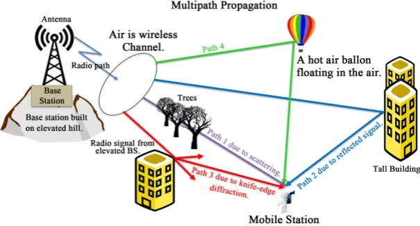
[image:2.595.222.525.542.705.2]Two significant forms of fading in cellular communications are multipath and shadow fading. Since cell phone users tend to move a lot, received signal strength fluctuates with these two multiplicative forms of fading [4]. In the out-door environment, shadow fading in cell phones causes long-term variation primarily caused by nearby mountains or tall buildings. Tall building structures shadow the radio signal, which results in a power drop at a receiver input. Mul-tipath, as illustrated in Figure 1, results in fluctuations of the signal amplitude because of the addition of signals that arrive with different phases [2].
Having an accurate estimate of the shadowing component of a received power signal will allow the mobile communication system to efficiently compensate for the signal degradation that will occur. As a result, it can help the system perform handoff at the most effective times (predict when and where to handoff user). In [5], the authors have presented and discussed the limitation of different types of windows-based estimators that are utilized to filter multipath noise from the in-stantaneous received power signal to estimate the local mean shadow power. Unfortunately, window-based estimators work well only under the assumption that the shadowing component is relatively constant during the window period. However, shadowing components are not constant; the fluctuations can vary and at times can significantly decrease the performance of the windows-based esti-mate. In [2], we proposed a second-order KF-based estimator as an alternative method to windows-based estimation for estimating local mean (shadow) pow-er.
Kalman filtering is a very effective algorithm that uses a series of measured observations and produces optimal estimates of states as explained in [6] [7] [8]. We applied this method to derive equations for an estimator that can estimate local mean (shadow) power profiles. In the initial stage of research, we used si-mulation models to validate the proposed method. The next challenge was to see if the model would work with real data. Therefore, in [1] we presented a new technique to experimentally characterize the wireless small-scale fading channel, taking into consideration real environmental conditions. This new two dimen-sional measurement technique provided essential information regarding the constructive and destructive interference patterns caused by the interaction be-tween the mobile station (while in motion) and surrounding obstacles. The two dimensional measurement technique enabled us to perform indoor experi- ments and collect real data, which we then used to confirm validation of the simulation model for the second-order KF-based estimator.Based on results from the indoor experiments, we concluded that the second-order KF-based es-timator is more accurate in predicting local mean (shadow) power profiles than the first-order KF-based estimator, even in channels with imposed non-Gaussian measurement noise.
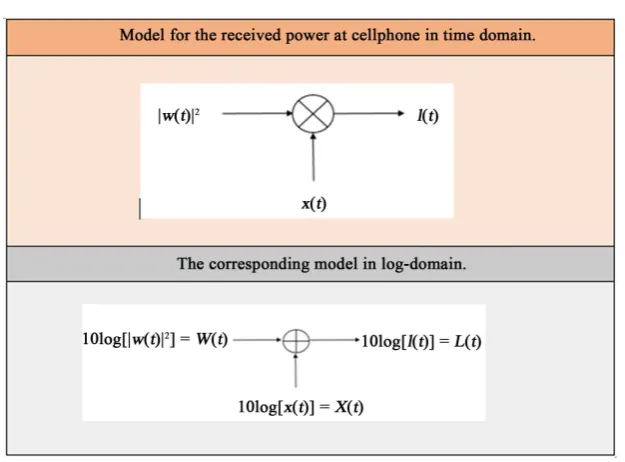
Figure 2. Model for the received power at cell phone.
2. Model for Multipath Signal
The description of Shadow Power Signal and its models as they pertain to our problem are presented in this section. In a wireless cellular radio environment, a model for an instantaneous received power signal l(t) at a cell phone is given in Figure 2, where
( )
2w t represents fast power fluctuation due to multipath and
x(t) represents slow power fluctuation due to shadowing. Many common sha-dow power estimation methods in industry rely on an accurate model for multi-path. Multipath is often modeled as Rayleigh noise for modeling purposes. It is customary to express power measurements in decibels. Handoff algorithms rely on estimates of shadow power in decibels [9].
To solve the problem, we start with the multipath model shown in Equation (2).
( )
( cos( )1 1) ( cos( )2 2) ( cos( ) )1 2
1
ej D t ej D t ej D Rt R
R
w R a a a
R
ω θ +φ ω θ +φ ω θ +φ
= + +
(1)
(
)
( )
( cos( 1) 1)1
1
1 e
1
D R R
j t
R
w R w R R a
R
ω θ+ +φ+
+
+ = ∗ +
+ (2)
where:
• v is the magnitude of the mobile velocity [10 m/s - 30 m/s],
•
λ
is the wavelength corresponding to the carrier frequency, which is typically 83 10
0.42 Hz 700 MHz
× =
,
• ωD is the Doppler spread equal to 2πv
λ . Range used here is [
2 π 10m s
3 Hz 7
∗ ∗
-
2 π 30m s
3 Hz 7
∗ ∗
],
• ar is gain [0 - 20],
• θr represents angles between incoming waves and mobile antenna. The value
range is uniformly distributed
[
−π, π]
. Other distributions like Normal can be used,•
{ }
1
R r r
φ = represents phase random variables whose values are also uniformly distributed
[
−π, π]
.3. Model for Shadow Power Signal
Equation (3) shows a widely accepted first-order state space model for the sha-dow process given by [10]. We derived a second-order state space model for the shadow process as shown in Equation (4).
1 1
k k k
x =a x− +φ (3)
2 2 1 1
k k k k
x =a x− +a x− +φ (4)
First shadow power coefficient a1 is given by Equation (5) and second
sha-dow power coefficient a2 is given by Equation (6):
1
1 e
s c
vT X
a −
= (5)
2
2 e
s c
vT X
a −
= (6)
where, v is the magnitude of the mobile velocity, Ts is time sample, and Xc
is effective correlation distance. The effective correlation distance is key attribute of the wireless environment. In urban area it can be as low as 10 m while in sub-urban areas it can be as high as 500 m. The effective correlation distance is given in Equation (7), where variable D is the distance between cell tower and cell phone measured in meters. Term εD is the correlation coefficient of shadow
process between two points separated by distance D.
( )
ln
c
D
D X
ε
− =
(7) Finally, system noise covariance is given in Equation (8), where term 2
s
σ
de-notes the shadow variance which depends on environment. In urban areas, typi-cal value for shadow variance is 4 dB while in suburban areas typitypi-cal value is 8 dB. Term φk in Equations (3) and (4) denotes zero mean white Gaussian noise
with variance 2
φ
σ
.(
)
2 1 2 2
s
a φ
σ = − ∗σ
(8)
4. Kalman Filter Algorithm
In this research, we applied the Kalman filter algorithm to estimate power signal in a mobile communication corrupted by multipath noise. The Kalman filter is a form of a linear algorithm for optimal recursive estimation of a system state with a specific set of output equations. The estimates are calculated every time a new measurement is received. Data received is processed sequentially, so it is not necessary to store the complete data set or to reprocess existing data when new measurement data is received.
4.1. Derivation of the Discrete-Time Linear Kalman Filter
This section derives the equations of the discrete-time Kalman filter. This filter is applied as a recursive solution to the estimation problem studied in this research. To use the Kalman filter to estimate signal of interest, one must first create ma-trices to fix the system model into a Kalman filter format. The following sets of equations describe the format of the linear discrete-time system:
1 1 1 1 1
k k k k k k
x =A x− − +B u− − +w− (9)
k k k k
y =H x +v (10)
The Kalman filter is a great tool, but its computation is complex and requires some explanation. An optimal value for xk in Equation (9) is calculated based
on the available knowledge of the system dynamics and the noise measurement
k
y . In Equation (10), yk represents the measured output of the system
(mea-surement of system state) with mea(mea-surement noise.
The k’s on the subscripts are states and can be treated as discrete time inter-vals. In general, when applying the Kalman Filter, the goal is to estimate state
k
x . For example, in signal processing, it is basically the estimate of some signal x that we want to find for each subsequent k. During this process, the Kalman fil-ter forms ana priori estimate and an a posterior estimate denoted as xˆk− and
ˆk
x+. Equation (11) computes the expected value of xk conditioned on all of the
measurement up to time k. Similarly, Equation (12) computes the expected value of xk conditioned on all of the measurements after time k.
[
| 1, 2, 3 1]
estimate of before the measurement at time is procces
ˆ
e ,
d ,
s
k k k
k
E x y y y
x y
x k
−
− =
=
(11)
[
| 1, 2, 3]
estimate of after the measurement at time is proccessed
ˆk k k
k
E x y
x y y y
x k
+= …
= (12)
Each system has to have initial values. Notation xˆ0
+ denotes an initial esti-mate of x0 before any measurements are taken. The first measurement in this
algorithm is taken at time k = 1. During this time period, the system does not have any measurements available to estimate x0, and therefore xˆ0
+ is formed as the best expected value of the initial state x0
( )
0 0
ˆ
x+=E x (13)
the true state and the estimated state. Therefore, the next step is to derive an er-ror equation. Equations (14) and (15) define an priori estimate error and an
posteriori estimate error, respectively.
ˆ
k k k
e−=x −x− (14)
ˆ
k k k
e+ =x −x+ (15)
Then, Equations (14) and (15) are used to compute covariance of the estima-tion error, which is denoted as Pk. The term
–
k
P denotes the covariance of the estimation error of xˆk−, and Pk+ denotes the covariance of the estimation error of xˆk+:
(
)(
)
Tˆ ˆ
k k xk k xk
P− E x − x −
− −
= (16)
(
)(
)
Tˆ ˆ
k k k k k
P+=E x −x+ x −x+ (17)
After the measurement at time k − 1 is processed, the estimate of the xk−1 is
computed, which is denoted as xˆk1 +
−. Also, the covariance of that estimate is computed at the same time, and it is denoted as Pk1
+
−. Then, at time k, before the measurement is processed, estimate of xk is computed and denoted as xˆk
−
Then, the covariance of these estimates are computed and denoted as Pk
− Then, at time k = 1, the measurement is processed to refine the estimate of xk. The
resulting improved estimates of xk and its covariance are denoted as xˆk
+ and
k
P+.
To begin the estimation process, initial values of the system determined in Equation (13) must be initialized. Then, with xˆ0
+, variable 1
ˆ
x− is computed using Equation (18). Based on this equation, the time update equation for xˆ is computed as indicated in Equation (19).
1 0 0 0 0
ˆ ˆ
x−=Ax++B u (18)
1 1 1 1
ˆk k ˆk k k
x−=A−x+− +B u− − (19)
From time
(
k−1)
+ to time( )
k −, the state estimate and its mean propagates the same way. As there are no additional measurements available between these two time-steps, the state estimate has to be updated based on a knowledge of system dynamics.Next step is to derive time-update equation for the covariance of the state es-timation error. The term P0
+ represents the covariance of the initial estimate of
0
x (the uncertainty in initial estimates of x0). If the exact value of the initial
state is known, then P0
+ can be set to zero. However, if the initial value is not known, then then P0 I
+= ∞ . The mathematical from for 0
P+ is shown in Equa-tion (20). The general descripEqua-tion of how the covariance of the state of a linear discrete-time system propagates with time is given by Equation (21). The term
– 1
P can be computed by substituting P0+ value from Equation (20). The time equation for term P in general form is given by Equation (23).
(
)(
)
T0 0 ˆ0 0 ˆ0
T
1 1 1 1
k k k k k
P =A P A− − − +Q− (21)
T
1 0 0 0 0
P−=A P F+ +Q (22)
T
1 1 1 1
k k k k k
P−=A P A− +− − +Q− (23)
Final step requires derivation of measurement-update equations for xˆ and P. Given xˆk− from Equation (19), we need to find a method to compute xˆk+, the
estimate of xk, which takes the measurement yk into account. Recall yk in
Equation (10) represents the measurement of the system state with measurement noise vk. Measurement noise is usually caused by the measurement instrument.
Based on the recursive least square estimation theory, we know that the availa-bility of yk changes the estimate of a constants x as follows:
(
)
1T T
1 1
k k k k k k k
K =P H− H P H− +R − (24)
(
)
1 1
ˆk ˆk Kk yk Hkˆk
x =x− + − x− (25)
(
)
(
)
(
)
(
)
T T 1 11 T 1
1
1
k k k k k k k k k
k k k k
k k k
P I K H P I K H K R K
P H R H
I K H P
− − − − − − = − − + = + = − (26)
where xˆk−1 and Pk−1 are estimates before the measurement is processed, while
ˆk
x and Pk take the measurements yk into account. The next step is to
re-write Equations (24) through (26) in a format that Kalman used when he derived his estimation theory. To formulate the measurement-update equations for xˆk
and Pk, simply perform the following substitutions: substitute xˆk−1 with xˆk
−,
1
k
P− with Pk−, xˆk with xˆk
+, and
k
P with Pk+. These substitutions lead to the following equations:
(
)
1T T
k k k k k k k
K =P H− H P H− +R − (27)
(
)
ˆk ˆk Kk yk Hkˆk
x+ =x−+ − x− (28)
(
) (
)
( )
(
)
T T 1 1 1k k k k k k k k k
T
k k k k
k k k
P I K H P I K H K R K
P H R H
I K H P
+ − − − − − − = − − + = + = −
(29)
The matrix Kk given in Equation (27) is called the Kalman filter gain. This
gain is a blending factor that minimizes the a posteriori error covariance. If the
k
x is a constant, then Ak =I, Qk =0, and uk=0.
The random variable wk represents process noise and vk represents
mea-surement noise. Terms vk and wk are independent of each other. They are
assumed to be white and with normal probability distributions
( )
(
0, k)
p w ∼N Q (30)
( )
(
0, k)
p v ∼N R (31)
In outdoor experiments, the process noise covariance matrix Qk and
4.2. First-Order Kalman Filter Application to Fading Channels
The Kalman Filter is a form of a linear algorithm for optimal recursive estima-tion of a system state with a specific set of output equaestima-tions. To build a simulator, understanding of system model and its dynamic behaviors is necessary. Then, the system must be represented in the state space format to be able to apply Kalman filtering. In other words, we need to mathematically model its states and parameters. This section presents set of equations used to create first-order KF-based estimator. References [10] and [11] were useful for programming in MATLAB during the initial stages of research.To build an estimation model in MATLAB, we started with equations intro-duced in Section 4.1 and substituted suitable entries from this problem to reflect the linear channel model [12]. Equations (9) and (10) can be rewritten as Equa-tions (32) and (33). This assumes a linear time invariant system with a mean of zero and white noise on both the state and output.
1 1 1
k k k k
x =Ax− +Bu− +w− (32)
k k k
l =Hx +v (33)
where:
• xk is a symbol value of shadow signal state that needs to be estimated. • uk is the control signal for handoff.
• wk is process white noise. • vk is measurement noise.
• lk is the measurement value for both shadow and multipath. In this docu-ment, lk or L(k) is the measurement value used to update shadow power
es-timate.
After initializing Kalman filter using initial values xO and PO as explained
in Section 4.1, time-update and measurement-update equations had to be identi-fied. These equations are computed for each time step k = 1, 2, 3. Equations (34) and (35) represent the “Time Update” state of the Kalman Filter, also known as the “Prediction States.” Equations (34) and (35) are derived by substituting suit-able entries from this problem into Equations (19) and (22). For first-order KF, matrix A was set to a1, which represents the first shadow power coefficient
given by Equation (5.5). Term for system noise covariance Qk in Equation (22),
was substituted with 2 φ
σ in Equation (35) and it denotes variance defined in Equation (34). Here we project the current state estimate forward in time with Equation (34) projecting the state ahead and Equation (35) projecting the error covariance ahead as represented below:
1 1
ˆk ˆk
x−=ax+− (34)
2
1 1
k k
P−=a P+− +σφ (35)
where xˆk− is the rough estimate before the measurement lk is processed at time k.
(37), (38) and (39) are derived by substituting suitable entries from this problem into Equations (27), (28) and (29). Here we adjust the projected estimate by an actual measurement at time k. Equation (37) was derived by substituting envi-ronment noise covariance Rk with
2
H
σ defined in Equation (36).
[
]
2
2
2 π 10 ln10
6
H
σ = (36)
Equation (37) computes the Kalman Gain, Equation (38) adjusts the projected estimate by an actual measurement lk, and Equation (39) updates the error
co-variance, as follows:
(
2)
1.
k k k H
K =P− P−+σ − (37)
If R is small and –
k
P is close to Identity, then Kk =HT
(
HHT)
−1, which is a well-known Pseudo inverse.ˆk
x : Estimate of x after the actual measurement lk at time k.
(
)
ˆk ˆk Kk k ˆk
x =x−+ l −x− (38)
(
1)
k k k
P+= −K P− (39)
The next step is to represent these estimates over a period of sufficient time. The output estimate in the previous step will be the input estimate in the next step. The main goal is to find an optimal value for xˆ .k
4.3. Second-Order Kalman Filter Application to Fading Channels
In this research, we assumed that the first-order state space model can be used to model Shadow Power. To extend the first-order state space model equations [1] presented in Section 4.2, a second-order state space model for the linear Kalman Filter was formulated and applied as suggested in the equations below. With this notation, we can describe an algorithm for the second-order KF as follows: • a1 is the first Shadow power coefficient as defined in Equation (5). • a2 is the second Shadow power coefficient as defined in Equation (6).• Xc is the effective correlation distance as defined in Equation (7).
• εD is the correlation coefficient of the shadow process between two points
separated by a distance D as measured in meters,
1
2
.
k k
k
x x
x
=
(40)
Equation (40) shows xk expressed in matrix format for second-order state
space.
Next set of equations present prediction states for second-order linear Kalman filter. Equation (34) can be rewritten as Equation (41). Therefore, Equation (41) in this section projects the state ahead, and Equation (43) projects the error co-variance ahead. For the second-order KF, the matrices are defined as follows:
1 2
1 0
k k
A
a a
=
,
0 0
B=
1 1 1
1 2 2 2
2
ˆ
1 0 0
ˆ ˆ 0 ˆ . k k k
k k k
k
x x
u
a a x
x − − − − = +
(41)
B is input matrix that relates the control input to the state xk. Matrix H is output equation whose function is to relate state to the measured output lk.
Parameter Q in Equation (42) represents the predicted process noise. Term
s
σ denotes the shadow variance with range from 4 dB to 8 dB. The notation
(
2)
21−a ∗σS in Equation (42) denotes the variance of the zero mean white Gaussian noise.
(
)
(
)
(
)
(
)
2 2 2 1 2 2 2 2 1 2 2 1 1 1 1 1 s s s sa a a
Q
a a a
σ σ σ σ − − = − − (42)
Equation (43) can then be expressed in the following state space format:
(
)
(
)
(
)
(
)
2 2 2 1 1 1 2 21 2 2
2 1 2 2 2 1 1 1
1 0 1
0 1 1
s s
k
k k
k k k s s
a a a
a
P P
a a a a a a
σ σ σ σ − + − − − = + − −
(43)
Next set of equations present correction states. Equation (44) was used to compute Kalman gain, which takes into consideration measurement noise due to multipath.
[
0 1]
H=
T 0
1
H =
(
)
1T T 2
k k k k k k H
K =P H− H P H− +σ − (44)
Equation (45) updates the estimate via lk, a measured value, and Equation
(46) updates the error covariance.
1 1 1
2 2 2
ˆ ˆ ˆ
ˆ ˆ ˆ
k k k
k k
k k k
x x x
K l H
x x x
+ − − + − − = + −
(45)
(
)
k k k
P+= I−K H P− (46)
*
X in Equation (47) is the optimal estimate of the second order shadow process. 1 * 2 ˆ ˆ k k x X H x =
(47) It is assumed that channel variation is mainly due to the changing mobile ve-locity and the correlation distance. Therefore, only the variation of the shadow process coefficient is considered. The smaller the sample period, the closer the shadow process coefficient is to one.
Figure 3. Block diagram of wireless communication system used in the outdoor experi- ment.
5. Outdoor Experiments
In [1], we presented a new technique to experimentally characterize the wireless small-scale fading channel, taking into consideration real environmental condi-tions. Then, using the technique that we described in [1], laboratory experiments were performed to collect real data and to validate the simulation model for the second-order KF-based estimator (designed to estimate power signal in cell phones). In [2], we showed that our simulation results in the MATLAB envi-ronment and laboratory experiment results validate the proposed algorithm and the theoretical analysis. We concluded that the second-order KF-based estimator is more accurate in predicting local shadow power profiles than the first-order KF-based estimator, even in channels with imposed non-Gaussian measurement noise. Next, we wanted to see how robust a second-order KF-based estimator is in the outdoor environment where we have different large-scale fading configu-rations. Therefore, outdoor experiments were set up as shown in Figure 3 to test a second-order KF-based model designed to estimate shadow power where wireless communication takes place while the user is in motion.
5.1. Measurements
A cell phone or portable phone uses radio waves to establish connection with its base station. Radio waves can travel long distances, but they easily get inter-rupted. As the transmitted signals travel from tower station to cell phone, they penetrate the atmosphere, and some signals are scattered, reflected, or observed. Objects obstructing the propagation path between the transmitter and receiver can cause variations in the received signal. All this can have a significant impact on signal strength in the cell phone device.
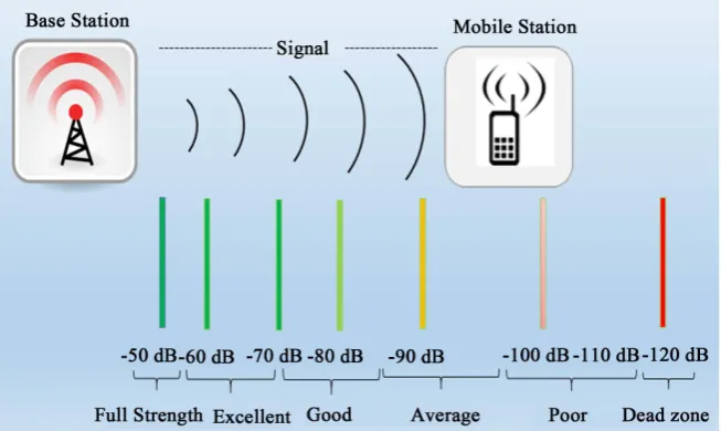
Figure 4. Cell phone signal strength range.
a measurement of the power present in a received radio signal. The higher the RSSI number, the stronger the signal. These values allow users to know when they are receiving a stronger signal or a weaker signal. Figure 4 shows that deci-bel values are expressed as negative numbers, which implies that the closer the value is to zero, the stronger the received signal. In Michigan, the standard fre-quency range for cellular phone operation is between −50 dB to −120 dB. User will get the best signal at −50 dB as it is considered full strength. On the other hand, −120 dB is considered a dead zone and the user will have no phone service. It also indicates that an ideal signal strength for optimum performance of a cell phone is about −65 dBm.
5.2. Field Test Scenario
Area or a region can impact signal strength or path loss. Therefore, as part of the experiment, we collected data in suburban and urban areas. Measurements have been conducted in two different environments while the user was driving a ve-hicle at different speeds:
1)Suburban environment, Oakland University campus in Auburn Hills, Michi-gan.
2)Urban environment, downtown Detroit, Michigan.
5.3. Outdoor Experiment Prerequisites and Setup
Cell phones work by communicating via radio waves using a system of cell towers that send and receive calls. A base station, also known as a cell tower, is placed on a big metal pole about 300 ft. high. Cell towers have triangular plat-forms on the top of the pole for cellular providers to keep their equipment. The process of a cell phone tower transmission requires the following equipment: ra-dios, antennas for receiving and transmitting radio frequency signals, compute-rized switching control equipment, GPS receivers, power sources, and some kind of protective cover. In this experiment, Verizon was the cellular provider and the location of the base station is shown in Figure 5.
A mobile station consists of the physical equipment (radio transceiver, dis-play and digital signal processors) and software package needed for communica-tion with a mobile network. In this experiment, the Samsung Galaxy S5 smart-phone was used as a mobile station. Any type of legal vehicle is acceptable to perform a driving test on public roads. As cell phone user moves around while using a cell phone, tall buildings will shadow the radio signal, which can result in a power drop at the receiver input. In this research, initial experiments were performed next to large buildings on the Oakland University campus to create a shadow fading phenomena in the outdoor environment. Supplementary experi-ments were conducted in downtown Detroit.
[image:14.595.237.511.515.702.2]Telecom tool that was released to the market by Wylisis in March 2017 is recommended for recording captured data (Figure 6) and vehicle movement. Telecom software has the capability to save logging data, which can be imported into MATLAB. Measured data includes cell tower location markers, signal strength, position, velocity, and time. Alternatively, the Data Acquisition Tool-box provides functions for connecting MATLAB to data acquisition hardware. Data can be analyzed as it is acquired or it can be saved for post-processing. Block diagram of wireless communication system used in the experiment setup outside of the lab environment is illustrated in Figure 3. The algorithm flow chart is presented in Figure 7.
Figure 6. Signal Strength measurement during outdoor experiment.
Figure 7. The algorithm flow chart.
5.4. Outdoor Experiment Results
This section presents outdoor experiment results for shadow process estimation and pertinent performance analysis. The purpose of these experiments was to study and analyze output results of the first-order state space model and to compare them to the second-order state space model while applying a Kalman Filter technique to determine shadow power signal in mobile communications from measurements that have impinged Rayleigh fast fading noise. As stated before, we were able to validate this concept through laboratory experiments with data from real scenarios, but those experiments performed in the indoor environment were limited by lower speed and obstacle contribution. The out-door experiment allowed us to conduct tests that include higher mobile velocity, exact shadow variance values, and large-scale fading configurations.
of data, but in this paper we include results from driving the vehicle at 36 mph in urban area as shown in Figure 7. The second-order KF-based estimator per-formed equally well when we varied the parameters.
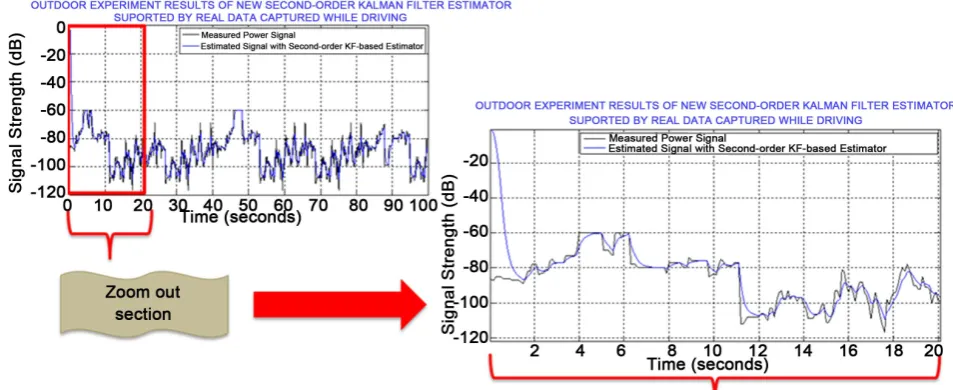
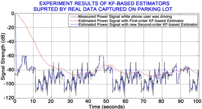
[image:16.595.212.536.286.465.2]The plots of outdoor experiment results supported by the field data are shown in Figures 8-10. These plots show results of the actual shadow power signal and estimations with Kalman Filtering. In Figure 8 and Figure 9, predicted power signal with the second-order KF-based estimator (marked in blue color) is very close to the measured signal (marked in black color). However, Figure 10 shows noticeable disparity between measured signal (marked in black color) and first- order KF estimate (marked in red color). These results clearly show that the second-order KF-based estimator tracks the actual shadow power more accu- rately than the first-order KF-based estimator. Average Error for the second- order KF-based estimator is lower than the first-order KF-based estimator. Also,
Figure 8. Power estimation in amobile station with asecond-order KF-based estimator using real data from the outdoor experiment.
[image:16.595.57.534.512.707.2]Figure 10. Comparison of system performance with the integrated second-order KF versus the same system with the first-order KF, which shows that the implementation of the second-order KF results in better estimation.
the second-order Kalman filter output has less lag from the actual shadow pow-er.
Authors in [5] presented results demonstrating that the first-order Kalman Filter method is superior to conventional window-based estimators like the sample average estimator, the uniformly minimum variance unbiased estimator, and the maximum likelihood estimator. Our results show that the second-order KF-based estimator improves the signal estimate significantly over the first-or- der KF estimate.
6. Conclusions
In this work, a second-order KF-based estimator has been further investigated in the outdoor environment, which is able to estimate local mean shadow power in mobile communications corrupted by multipath noise. In our experiments, we mainly explored how the second-order KF-based estimator compares to the first-order KF-based estimator. Based on our results from the indoor experi-ments of small-scale fading presented in [2], we concluded that the second-order KF-based estimator is more accurate in predicting local mean (shadow) power profiles than the first-order KF-based estimator, even in channels with imposed non-Gaussian measurement noise. To fully complete the proposed theory, we recently extended the research to the outdoor environment and compared how these two estimators handled variability due to higher vehicle speed, larger dis-tances, and distant large objects in the outdoor environment, such as mountains or large buildings. A Telecom tool/software released to market in 2017 was used to measure cell phone signal strength and other key parameters outside of the lab environment. Signal measurements have been conducted in typical environ-ments like urban and suburban areas.
results supported by field data are provided in Figures 8-10. These plots clearly show that the second-order Kalman filter tracks the actual shadow power more accurately than the first-order Kalman filter. The system was able to operate without a failure under variety of conditions, which demonstrates model ro-bustness. With MATLAB software, we were able to efficiently explore, analyze, and visualize measured data from the outdoor experiment. Comparison analysis was performed as explained in [11] [12]. Simulations in the MATLAB environ-ment, laboratory, and outdoor experiment results have been consistent in showing that our implementation of the second-order KF results in better estimation.
7. Future Work
Math Works currently offers some basic examples of Kalman Filter theory. Therefore, we will most likely share our code for a first-order KF-based estima-tor and second-order KF-based estimaestima-tor by deploying an Application with MATLAB, so others can use it too. According to MathWorks’ web site, there is a wide range of options for deploying and sharing an application that was devel-oped in MATLAB. As future work, we will look into these options.
When the channel is nonlinear, the Unscented Kalman filter also can be ap-plied to the state space model to further improve and optimize the shadow pow-er presented in this pappow-er. The Unscented Kalman filtpow-er is popular due to its su-periority in approximating and estimating nonlinear systems and its ability to handle non-Gaussian noise environments [13]. We may consider this optimiza-tion in the future.
As future work, we also are considering designing a third-order KF-based es-timator. When the order of the filter is higher, we predict that there will be bet-ter noise repair. However, there is a tradeoff between three things: order of filbet-ter, computational difficulty of filter, and accuracy. Therefore, we need to look at these to determine if higher order estimators are practical.
Acknowledgements
The authors would like to express appreciation to Eric Yaharmatter from Auto-liv Inc. for his initial thoughts on this subject.
Conflict of Interest
The authors declare that they have no conflict of interest.
References
[1] Mawari, R., Henderson, A., Akbar, M., Dargin, G. and Zohdy, M. (2016) ) An Im-proved Characterization of Small Scale Fading Based on 2D Measurements and Modeling of a Moving Receiver in an Indoor Environment. Journal of Signal and Information Processing, 7, 160-174. https://doi.org/10.4236/jsip.2016.73016
In-formation Processing, 7, 61-74. https://doi.org/10.4236/jsip.2016.72008 [3] Graf, Z. (1974) Dictionary of Electronics.
[4] Yarhmatter, E. and Kapetanovic, A. (2012) Power Estimation in Mobile Communi-cations: Comparison of the First Order AR Model to Second Order AR Model. Oakland University, Rochester, MI. (Unpublished)
[5] Jiang, T., Sidiropoulos, N.D. and Giannakis, G.B. (2003) Kalman Filtering for Power Estimation in Mobile Communications, IEEE Transactions on Wireless Communi-cations, 2,151-161. https://doi.org/10.1109/TWC.2002.806386
[6] Kalman, R.E. (1960) A New Approach to Linear Filtering and Prediction Problems. Research Institute for Advanced Study, Baltimore.
[7] Simon, D. (2006) Optimal State Estimation: Kalman, H∞ and Nonlinear Approach-es. 1st Edition, John Wiley & Sons Inc., New Jersey.
https://doi.org/10.1002/0470045345
[8] Nsour, A., Abdallah, A.-S. and Zohdy, M. (2013) An Investigation into Using Kal-man Filtering for Phase Estimation in Bluetooth Receivers for Gaussian and Non-Gaussian Noise. 2013 IEEE International Conference on Electro/Information Technology, Rapid City, 9-11 May 2013, 1-5.
https://doi.org/10.1109/EIT.2013.6632644
[9] Rappaport, T.S. (2010) Wireless Communications Principles and Practice. 2nd
Edi-tion, Persons EducaEdi-tion, London.
[10] Gudmundson, M. (1991) Correlation Model for Shadowing Fading in Mobile Radio Systems. Electronics Letters, 27, 2145-2146. https://doi.org/10.1049/el:19911328 [11] Grewal, M.S. and Andrews, A.P. (2014) Kalman Filtering Theory and Practice
Us-ing MATLAB. 4th Edition, John Wiley & Sons Inc., New York.
[12] Brown, R.G. and Hwang, P.Y.C. (2012) Introduction to Random Signals and Ap-plied Kalman Filtering with Matlab Exercises. 4th Edition, John Wiley & Sons Inc., Hoboken.
[13] Li, L. and Xia, Y. (2013) Unscented Kalman Filter over Unreliable Communication Networks with Markovian Packet Dropouts. IEEE Transactions of Automatic Con-trol, 58, 3224-3230. https://doi.org/10.1109/TAC.2013.2263650
Submit or recommend next manuscript to SCIRP and we will provide best service for you:
Accepting pre-submission inquiries through Email, Facebook, LinkedIn, Twitter, etc. A wide selection of journals (inclusive of 9 subjects, more than 200 journals)
Providing 24-hour high-quality service User-friendly online submission system Fair and swift peer-review system
Efficient typesetting and proofreading procedure
Display of the result of downloads and visits, as well as the number of cited articles Maximum dissemination of your research work