Abstract—The optimum grinding parameters have always been important in producing the best surface finished workpiece. A parameter deemed essential for obtaining an excellent surface finish is the use of liquid coolant. Unfortunately, large quantities of liquid waste are produced by its use, and it is now imperative that companies implement appropriate waste disposal measures. To date, there have only been a limited numbers of investigations of other methods which do not rely on liquid coolant. Alternative strategies which do not rely on liquid coolant will still require that the ground workpiece is produced to similar surface finish. The goal of this research is to reduce the reliance on liquid coolant, while still producing a suitable standard workpiece.
Index Terms—Optimum grinding parameters, liquid coolant, waste disposal, cold air, Taguchi method
I. INTRODUCTION
raditionally the grinding of hard materials requires the application of copious amounts of coolant to dissipate the generated heat, and to help provide an excellent finish to the workpiece [1, 2]. Unfortunately, the vast quantities of liquid waste produced is environmentally damaging and requires appropriate waste disposal procedures [3]. Typically the waste produced by grinding consists of metal chips and coolant, plus the less obvious amount of greenhouse gas produced by the coolant pump motor [4]. The technique used for assessing the environmental impact associated with grinding is performed in accordance with the Environmental Management Life Cycle Assessment Principles and Framework ISO 14040 standard [5]. Dry grinding is obviously more environmentally acceptable as there are no disposal issues to consider. For this reason liquid coolant is replaced by cold air [6]. The challenge that is now faced is how to find the optimum grinding conditions to produce parts cooled by cold air. To help achieve this goal the Taguchi Method was used to establish the best parameters to produce a workpiece to the required quality [7]. A three level L27 orthogonal array was selected where 0, 1 and 2 represent the different control levels, dry,
Manuscript received February 29, 2016; revised March 22, 2016. Grinding Using Cold Air Cooling
Brian Boswell is a Lecturer at Curtin University Perth Western Australia 6845, corresponding author phone: +61 8 9266 3803; fax: +61 8 9266 2681; (e-mail: b.boswell@ curtin.edu.au)
Mohammad Nazrul Islam is a senior Lecturer at Curtin University Perth
Western Australia (e-mail: [email protected]).
Jong Chua Ong was a student at Curtin University Perth Western Australia
(e-mail: [email protected]).
Yogie R. Ginting is a Lecturer at University of Riau Pekanbaru Indonesia (e-mail: [email protected]).
cold air and flood.
Analysis of the tests provided the deviation and nominal values of the quality measurements used to determine the optimum grinding process (cutting force and surface roughness). Further analysis implemented the use of signal-to-noise ratios to differentiate the mean value of the experimental tests and nominal data of these quality measurements. A viable measure of detectability of a flaw is its signal-to-noise ratio (S/N). Signal-to-noise ratio measures how the signal from the defect compares to other background noise [8]. The signal-to-noise ratio classifies quality into three distinct categories and the noise ratio differs with each category. The three different formulas are given below [9];
∑
=−
=
nn i
i
y
n
N
S
1
2log
10
[dB] (1)
=
s
yy
N
S
2 _
log
10
[dB] (2)∑
=−
=
nn i
i
y
n
N
S
2
1
1
log
10
[dB] (3)The results from this formula suggest that the greater the magnitude of the signal-to-noise ratio, the better the result will be because it yields the best quality with least variance [10]. The signal-to-noise ratio for each of the quality measurements was calculated, and the mean signal-to-noise ratio for each parameter was found and tabulated. The results were graphed to illustrate the relationship that exists between S/N ratio and the input parameters at different levels. The gradient of the graph represented the strength of the relationship for each of the grinding parameters.
To help analyse the contribution of each variable and their interactions in terms of quality, the Pareto ANOVA analysis is implemented. The Pareto ANOVA analysis was completed for each of the quality measures: force, and surface roughness. The Pareto ANOVA analysis identified which control parameter affected the quality of the ground workpiece. By using the Pareto principle only 20% of the total grinding configuration is now required to generate 80% of the benefit of completing all machining test configurations [11]. This method separates the total variation of the S/N ratios.
II. GRINDING LITERATURE REVIEW
Grinding was discovered more than 2000 years ago, when abrasive stones were used for sharpening knives and tools
Grinding Using Cold Air Cooling
B. Boswell, M. N. Islam, Member IAENG, Y. R. Ginting Member IAENG and J. C. Ong
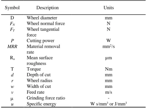
[12]. Material Removal Rate (MRR), is easily defined as the rate of removal of the material from the surface of the workpiece when coming into contact with the unit width of the grinding abrasive. Table I gives the nomenclature for the equations used for surface grinding, Kalpakjian and Schmid [13] used equation (4) to calculate MRR.
[image:2.595.372.482.100.235.2]MRR = dwv (4) (1)
TABLE I
Nomenclature For Surface Grinding
Symbol Description Units
D Wheel diameter mm
FN Wheel normal force N
FT Wheel tangential
force
N
P Cutting power W
MRR Material removal
rate
mm2/s
Ra Mean surface
roughness
µm
T Torque Nm
d Depth of cut mm
r Wheel radius mm
w Width of cut mm
v Feed rate m/s
µ Grinding force ratio -
u Specific energy W s/mm3 or J/mm3
However, when the grinding process requires a higher MRR, it causes higher stresses on the grinding wheel abrasive [14]. This would not only cause the pores of the grinding wheel to get clogged up, but also require constant dressing. A newer grinding method, known as High Efficiency Deep Grinding (HEDG), tends to reduce the cost of manufacturing by increasing the material removal rate by almost 300 times [15]. Specific energy (u), provides a valuable measure of the grinding wheel’s ability to remove material [14]. It is also defined by Kalpakjian and Schmid [13] as the energy per unit volume of material ground from the workpiece surface. In order to properly determine the specific energy of a certain material, the sharpness of the grinding wheel and the grindability of the workpiece have to be taken into account, as the specific energy mostly depends on those two variables. To calculate the specific energy, the following equation can be used.
MRR
P
u
=
(5)Typically, a specific energy range for grinding would range from 15 – 700J/mm2 [14]. This range is normally higher than other machining operations, e.g. turning or milling, where the specific energy ranges from 0.4 – 5J/mm2 [13]. This is due to the presence of wear for other machining processes. Determining the grinding forces is crucial when estimating the power requirements, as it helps with the design of grinding machines, fixtures and work-holding devices [13]. This is important for high accuracy operations, minimising deflection of workpiece and ensuring dimensional accuracy [13].
There are three different types of grinding forces: tangential/cutting, normal/thrust and axial force that act on a grinding wheel [14]. The thrust force (FN) is the force of
the grinding wheel acting perpendicular to the work piece, while the cutting force, FT acts parallel to the work piece as shown in Fig. 1.
Fig. 1. Acting Forces.
In order to acquire the tangential force, the equation (6) acquired from Kalpakjian and Schmid [13] can be used.
MRR
P
u
=
(6)Normally the thrust force is assumed to be 30% higher than the tangential cutting force, as acquired from technical literatures [13]. The thrust force used in this work was obtained via an experimental process, and should be noted that the data acquired was greater than 30%. The grinding force ratio (µ) was used to get indirect information with regards to the efficiency of the grinding operations. This used the measured forces as given by equation (7).
N T
F
F
=
µ
(7) [image:2.595.45.283.176.350.2]
that create a grinding wheel, the abrasive grain, bond and porosity.
Fig. 2a. Grinding Wheel Structure [13].
When choosing a conventional abrasive grinding wheel from a manufacturer, it is usually selected by using the standard marking shown in Fig. 2b below.
I II III IV V VI VII
51 - A - 36 - L - 5 - V - 23
Fig. 2b. Typical grinding wheel code.
These numbers and symbols determine the grit, porosity and grade for a grinding wheel.
III. Grinding Tests and Set-Up
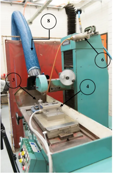
[image:3.595.47.291.80.150.2]This work was performed by using a surface grinder fitted with an extractor for removing the dry particles of swarf as they fly off the grinding wheel. Table II lists the description and model numbers of the equipment used for the grinding test. The AISI 1045 carbon steel workpiece was securely clamped to the dynamometer, which in turn was secured to the magnetic table as shown in Fig. 3. The force measurements given by the Dynoware28 software produced real-time graphics of the cutting forces, and is used for analysing the process, with the tests being repeated three times each to ensure the robustness of test data.
TABLE II Test Equipment Used
Part Brand Model Description
1 Abwood HS 5025 Surface Grinder
2 Norton BV200778
Aluminium Oxide - Medium Grit - Grinding Wheel -
38A60JVBE
3 - - Multipoint Dresser – Matrix
Style
4 Kistler 9257BA Dynamometer
5 Kistler 5233A Control Unit
6 AiRTX 21025 Vortex Tube
7 - AISI 1045 Medium Carbon Steel Work
piece
8 Plymoth P-001 Vacuum
9 Mitutoyo SJ-201 Surface Roughness Tester
Fig. 3. Workpiece clamped onto dynamometer.
A Mitutoyo Surftest portable stylus type surface roughness tester was used to measure the surface quality of the workpieces. The ideal roughness represents the best possible finish which can be obtained for a given grinding condition. The surface roughness produced by the previously mentioned parameters would usually be found as:
• cracks due to thermal impact, • craters from grain fractures, • not using cutting fluids
• traverse and longitudinal waves that are all caused by the random nature during the grinding process or due to machine vibrations [16].
Cold air was provided by a Vortex Tube (VT), which is a simple device, which has no moving parts, and only needs a steady stream of high-pressure compressed air [17]. This is provided by the high pressured air entering the VT generator where it reaches a high angular velocity which subsequently causes a vortex-type of flow in the tube. By adjusting the hot exit it is possible to vary the flow and temperature of the air that leaves through the cold exit.
The grinding tests were planned using the design of experiment (DOE) methodology for a three level, three parameter experiment array [18]. A total of 27 grinding conditions were tested three times each. All the non-varying variables were fixed and setup at a constant value as per Table III. Subsequently, dressing was done for every workpiece, giving a new layer of unclogged abrasive grains.
6
4 3
[image:3.595.43.297.238.288.2]After which the grinding wheel was passed across the workpiece a few times at a depth of 2 - 4µm to ensure a true DOC for the tests.
TABLE III Fixed Parameters
Feed Rate (f) 73mm/s
Wheel Speed (N) 2600 rpm
Air Pressure Going into
Vortex Tube 75 psi
Grinding Wheel
Diameter (D) 170mm
Having now eliminated any high points on the grinding wheel, the subsequent grinding tests could be carried out. Before dry or air cooling the grinding wheel was allowed to run until all previous cutting fluid had dissipated. The dynamometer was mounted square to the grinding wheel and parallel with the magnetic chuck. Once secured to the dynamometer, a diamond dresser, part 3 in Fig. 3, was then attached onto the magnetic chuck, away from the dynamometer. The diamond dresser was placed at the corner of the magnetic chuck in order to not interfere with the tests, and to minimise the need to remove and align the dynamometer every time the grinding wheel needs to be dressed. A copper tube was attached to the cold air exit of the VT and directly onto the grinding wheel and workpiece. As there is no liquid cutting fluid to capture the fine metal swarf particles, a vacuum as shown in Fig. 3 part 8, was placed directly opposite the cold air exit, on the other side of the grinding wheel. This precaution was employed to prevent any of the fine metal particles being blown into the atmosphere, ensuring a safe working area. The grinding test control parameters used for surface grinding the workpieces are given in Table IV.
TABLE IV
Control Parameters and their Levels Control
Parameters Units Symbol
Levels
Level 0 Level 1 Level 2
Cooling Method
- A Dry Cold
Air
Flood
Width of Cut mm B 5 10 15
Depth of Cut µm C 5 10 15
[image:4.595.294.557.148.709.2]Before performing any experimental work the VT was turned on and left running for around 15 minutes in order for the air to cool down to a constant temperature. Thermocouples monitored the temperature of the VT cold air and the ambient temperature as given in Table V.
TABLE V
Temperatures of Ambient and Vortex Cold Air
Ambient Air 20 – 22oC
VT Output Air -8oC
The Dry grinding test width of cut were 5, 10 and 15mm, with the depth of cut being maintained at 5, 10 and 15µm for each test.
III. RESULTS AND DISCUSSION
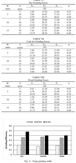
Each of the grinding test conditions were used three times, and the average of the cutting and thrust force from the
grinding tests are tabulated in Table VI, VII and VIII respectively. An example of a graph of grinding efficiency with respect to cooling method for the 15mm width of cut is shown in Fig. 4, which indicated that cold air was close to that of flood cooling, over the tested range. For the 5 and 10mm width of cuts the air cooling, indicated cold air to be acceptable for workshop use.
TABLE VI Dry Grinding Forces W
(mm)
d (µm)
FT FN Fr µ
(N)
5
5 2.82 12.50 12.82 0.23
10 5.06 16.67 17.42 0.31
15 9.78 24.75 26.61 0.40
10
5 2.08 10.86 11.06 0.19
10 7.76 20.35 21.78 0.38
15 11.81 27.29 29.74 0.43
15
5 2.78 13.62 13.90 0.20
10 7.83 21.43 22.81 0.36
15 13.57 28.76 31.80 0.48
TABLE VII Cold Air Grinding Forces W
(mm)
d
(µm))
FT FN Fr µ
(N)
5
5 1.04 11.15 11.20 0.13
10 5.07 17.84 18.55 0.28
15 11.18 27.37 29.57 0.41
10
5 3.61 14.62 15.06 0.24
10 7.50 21.99 23.24 0.34
15 10.82 26.13 28.28 0.41
15
5 2.34 13.21 13.42 0.17
10 6.90 18.73 19.96 0.37
15 9.60 24.06 25.92 0.40
TABLE VIII Flood Grinding Forces W
(mm)
d
(µm)
FT FN Fr µ
(N)
5
5 0.41 12.28 12.28 0.03
10 6.78 20.51 21.60 0.32
15 10.56 26.91 28.91 0.39
10
5 1.26 12.29 12.35 0.13
10 3.37 13.16 13.58 0.25
15 11.85 28.25 30.63 0.42
15
5 2.79 14.12 14.39 0.19
10 8.80 25.01 26.51 0.35
15 11.72 29.55 31.79 0.40
0 0.1 0.2 0.3 0.4 0.5 0.6 Gr indi ng E ff ic enc y
Dry Cold Air Flood 5 mm 10 mm 15 mm
Fig. 4. 15mm grinding width.
[image:4.595.91.249.631.674.2]approximately 50% higher than that stated by Kalpakjian and Schmid [13]. The thrust force, normally assumed to be 30% higher than the cutting force, was found to be the case for all tests.
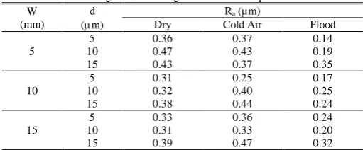
[image:5.595.40.296.163.269.2]Table IX below gives the average surface roughness for the grinding tests at a width of cut of 5, 10 and 15mm respectively.
TABLE IX
Average Surface Roughness of the Workpieces W
(mm)
d
(µm)
Ra (µm)
Dry Cold Air Flood
5
5 0.36 0.37 0.14
10 0.47 0.43 0.19
15 0.43 0.37 0.35
10
5 0.31 0.25 0.17
10 0.32 0.40 0.25
15 0.38 0.44 0.24
15
5 0.33 0.36 0.24
10 0.31 0.33 0.20
15 0.39 0.47 0.32
The workpiece surface roughness from Table IX shows that all of the surface roughness for the dry, cold air and flood grinding operations fell well within the standard expected for this process Table X. For the traditional flood grinding at 5 and 10µm DOC respectively, the surface roughness obtained was between 0.14 to 0.25µm, i.e. in the lower area for standard surface grinding finishes.
TABLE X
Surface Roughness Data for Grinding Obtained from Machinery’s Handbook [19]
Process Roughness Average Ra
25 12.5 6.3 3.2 1.6 0.8 0.4 0.2 0.1 0.05 0.025 0.01
Grinding
Comparing the cold air with dry grinding the surface roughness was found to be in all extents similar to dry grinding. The grinding test data conclusively shows that the better surface roughness values were obtained when cutting fluid was used. As expected the surface finish data increased generally with the deeper DOC. Comparing the cold air and dry grinding surface roughness, the cold air surface roughness was shown to be slightly worse than that of the dry grinding. As cold air was used there was no lubrication, and any broken off abrasive grits may have traveled along the surface of the workpiece. This in turn, increased the microscopic scratching on the surface.
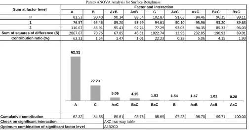
The Signal to Noise ratio (S/N) Analysis and the Pareto Analysis of Variance (ANOVA) depicts how the 27 different combinations of testing parameters have an effect on the surface finish, and forces on the ground workpiece was also revealed. (The strong interactions between the testing parameters.) Using the Pareto ANOVA the optimum combination was determined for the optimum grinding force and surface finish, with respect to width, DOC and cooling method. The Pareto ANOVA analysis Table XI showed that parameter A (cooling method) had the most significant effect on surface roughness (P = 62.32%), followed by C (DOC, P = 22.23%) and B (width of cut, P = 1.54%). The A×C interaction (cooling type and DOC) also played a role in the grinding process, with P = 5.06%. The total contribution by the interactions was approximately 40% making it difficult to be definitive on the benefits of
air cooling. The results obtained from the Pareto ANOVA analysis in Table XI are verified by the response as given in the response graph Fig. 8 for the mean S/N ratio. From Table XI it is found that the optimum combination for surface roughness that can be used in a grinding operation is (A2B1C0) i.e. the combination of the traditional grinding operation at 10mm width of cut and a 5µm DOC. However, from Table XII, the optimum force the combination is (A1B0C0) i.e. cold air, 5mm width cut and 5µm DOC. The results show that the optimum combination to achieve the best surface roughness is (A2B1C0); i.e. Flood, 10mm width, and lowest DOC.
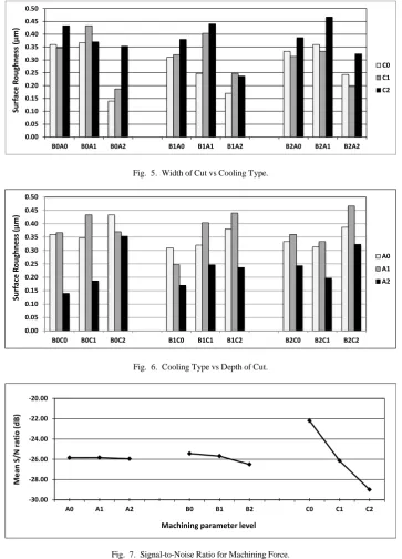
Additional traditional analysis of the surface finish with respect to a cooling method is shown in Fig. 5 and 6, which was used to verify the Pareto ANOVA and Taguchi’s S/N analysis. As illustrated in Fig. 5, the best surface grinding is achieved at (A2B1) flood cooling, and 10mm width of cut with similar agreement for DOC Fig. 6. The results therefore confirm those obtained from the Pareto ANOVA and Taguchi S/N in terms of cooling method. However, for air cooling the results are non-conclusive from Fig. 5, for the best surface finish conditions. Fig. 6 indicates the best parameters for obtaining a good surface finish with respect to (C0B1) low DOC and 10mm width of cut as also shown by Table XI.
IV. CONCLUSION
The test data proved that the cold air alternative cooling methods being trialed were not effective over the whole range of grinding parameters. Even with this statement cold air from a VT can still be considered as an important method of cooling and should be implemented more in industry. The surface roughness that was obtained during the grinding tests was all well within the range of standard grinding operations. The justification for using cold air is that there is no contaminated liquid coolant to be processed, and the grinding efficiency was compatible with flood cooling Fig. 4. Additional power saved by not having a coolant pump running constantly as compressed air would only be used as needed. Use of cold air implies the principles of good environmental management is being sought as expressed by the ISO 14040 framework.
grit cutting edge. This was shown to be effective by the work carried out by Sanchez et al. [21], where MQL and CO2 was used as the coolant. The disadvantage of the approach was by the use of CO2 as it is a greenhouse gas. Interestingly the force data from the tests showed that the thrust force measurement’s did not prove the normal convention as stated by Kalpakjian and Schmid [13] i.e. to be 30% higher than the cutting force. This is worthy of further investigation.
REFERENCES
[1] Y. Gao, H. Lai, and S. Tse, "Effects of actively cooled coolant for
grinding brittle materials," in Key Engineering Materials, 2005,
pp. 233-238.
[2] Y. Gao and H. Lai, "Effects of actively cooled coolant for grinding
ductile materials," in Key Engineering Materials, 2007, pp.
427-433.
[3] J. P. Davim, Green manufacturing processes and systems:
Springer, 2013.
[4] T. Gutowski, C. Murphy, D.Allen, D.Bauer, B. Bras, T. Piwonka,
et al., "Environmentally Benign Manufacturing: Observations
from Japan, Europ and United States," Jounal of Cleaner
Production, vol. 13, pp. 1-17, 2005.
[5] A. N. I. 14040, "Environmental management Life cycle
assessment Principles and framwork," ed. 1 The Crescent, Homebush NSW 2140 Australia: Standards Australia and Standards New Zealand, 1998.
[6] P. S. Sreejith and B. K. A. Ngoi, "Dry Machining: Machining of
The Future," Journal of Materials Processing Technology, vol.
101, pp. 287-291, 4/14/ 2000.
[7] R. K. Roy, A primer on the Taguchi method: Society of
Manufacturing Engineers, 2010.
[8] R. Roy, A Primer on the Taguchi Method: Society of
Manufacturing Engineers, 1990.
[9] S. Tanaydin, "Robust Design and Analysis for Quality
Engineering," Technometrics, vol. 40, p. 348, 1998.
[10] N. H. Rafai, "An investigation into dimensional accuracy and
surface finish achievable in dry turning," Machining science and
technology, vol. 13, p. 571, 2009.
[11] D. Haughey. (2013). Pareto Analysis Step by Step. Available:
http://www.projectsmart.co.uk/pareto-analysis-step-by-step.html
[12] R. A. Irani, R. J. Bauer, and A. Warkentin, "A Review of Cutting
Fluid Application in The Grinding Process," International
Journal of Machine Tools and Manufacture, vol. 45, pp. 1696-1705, 2005.
[13] S. Kalpakjian and S. R. Schmid, Manufacturing Engineering and
Technology, 6th ed. Singapore: Prentice Hall, 2006.
[14] W. B. Rowe, Principles of Modern Grinding Technology, 1st ed.
Oxford: William Andrew, 2009.
[15] D. Babic, D. B. Murray, and A. A. Torrance, "Mist Jet Cooling of
Grinding Processes," International Journal of Machine Tools
and Manufacture, vol. 45, pp. 1171-1177, 2005.
[16] R. L. Hecker and S. Y. Liang, "Predictive Modeling of Surface
Roughness in Grinding," International Journal of Machine Tools
& Manufacture, vol. 43, pp. 755-761, 2003.
[17] N. F. Aljuwayhel, G. F. Nellis, and S. A. Klein, "Parametric and
internal study of the vortex tube using a CFD model,"
International Journal of Refrigeration, pp. 442-450, 2004.
[18] R. K. Roy, Design of experiments using the Taguchi approach:
16 steps to product and process improvement: John Wiley & Sons, 2001.
[19] E. Oberg, Section 11. Machine Elements–Machinery’s
Handbook 29: Industrial Press, 2012.
[20] J.-S. Kwak, "Application of Taguchi and Response Surface
Methodologies for Geometric Error in Surface Grinding Process,"
International Journal of Machine Tools & Manufacture, vol. 45, pp. 327-334, 2005.
[21] J. A. Sanchez, I. Pombo, R. Alberdi, B. Izquierdo, N. Ortega, S.
Plaza, et al., "Machining evaluation of a hybrid MQL-CO2
grinding technology," Journal of Cleaner Production, vol. 18, pp.
0.00 0.05 0.10 0.15 0.20 0.25 0.30 0.35 0.40 0.45 0.50
B0A0 B0A1 B0A2 B1A0 B1A1 B1A2 B2A0 B2A1 B2A2
Su
rf
ac
e
Ro
ug
hn
es
s (
μm
)
C0 C1 C2
Fig. 5. Width of Cut vs Cooling Type.
0.00 0.05 0.10 0.15 0.20 0.25 0.30 0.35 0.40 0.45 0.50
B0C0 B0C1 B0C2 B1C0 B1C1 B1C2 B2C0 B2C1 B2C2
Su
rf
ac
e
Ro
ug
hn
es
s (
μm
)
A0 A1 A2
Fig. 6. Cooling Type vs Depth of Cut.
-30.00 -28.00 -26.00 -24.00 -22.00 -20.00
A0 A1 A2 B0 B1 B2 C0 C1 C2
M
ean
S
/N
ra
tio
(d
B)
[image:7.595.116.480.86.591.2]Machining parameter level
Fig. 7. Signal-to-Noise Ratio for Machining Force.
6.00 8.00 10.00 12.00 14.00
A0 A1 A2 B0 B1 B2 C0 C1 C2
M
ean
S
/N
ra
tio
(d
B)
[image:7.595.121.477.88.226.2]Machining parameter level
Table XI
Pareto ANOVA Analysis for Surface Roughness
A B AxB AxB C AxC AxC BxC BxC
81.53 90.40 90.14 88.54 102.87 91.63 84.46 96.25 89.11 76.57 95.46 89.20 93.99 94.61 90.10 95.96 93.20 89.63 116.67 88.91 95.43 92.24 77.29 93.03 94.35 85.32 96.03 2867.67 70.76 67.85 46.51 1022.74 12.95 232.85 190.93 89.01 62.32 1.54 1.47 1.01 22.23 0.28 5.06 4.15 1.93
62.32 84.55 89.61 93.76 95.69 97.23 98.70 99.71 100.00
Check on significant interaction
Optimum combination of significant factor level A2B2C0
AXC two-way table
Sum at factor level Factor and interaction
0 1 2
Sum of squares of difference (S) Contribution ratio (%)
Cumulative contribution
62.32
22.23
5.06 4.15 1.93
1.54 1.47 1.01 0.28
[image:8.595.48.548.372.643.2]A C AxC BxC BxC B AxB AxB AxC
TABLE XII
Pareto ANOVA Analysis for Machining Force
A B AxB AxB C AxC AxC BxC BxC
-232.66 -228.95 -226.53 -237.07 -199.78 -230.43 -233.58 -234.79 -230.05 -232.52 -231.24 -234.56 -231.64 -235.27 -234.84 -232.26 -231.52 -233.68 -233.60 -238.59 -237.69 -230.07 -263.73 -233.51 -232.94 -232.47 -235.04 2.10 152.20 198.67 81.12 6159.71 30.60 2.60 17.04 39.95 0.03 2.28 2.97 1.21 92.16 0.46 0.04 0.25 0.60
92.16 95.13 97.41 98.62 99.22 99.68 99.93 99.97 100.00
Check on significant interaction
Optimum combination of significant factor level A1B0C0
AXB two-way table
Sum at factor level Factor and interaction
0
1 2
Sum of squares of difference (S) Contribution ratio (%)
Cumulative contribution
92.16
2.97 2.28 1.21 0.60 0.46 0.25 0.04 0.03