ISSN Online: 2153-120X ISSN Print: 2153-1196
DOI: 10.4236/jmp.2019.1011091 Oct. 23, 2019 1374 Journal of Modern Physics
A Formulation of Spin Dynamics Using
Schrödinger Equation
Vu B. Ho
Advanced Study, 9 Adela Court, Mulgrave, Australia
Abstract
In quantum mechanics, there is a profound distinction between orbital angu-lar momentum and spin anguangu-lar momentum in which the former can be as-sociated with the motion of a physical object in space but the latter cannot. The difference leads to a radical deviation in the formulation of their corres-ponding dynamics in which an orbital angular momentum can be described by using a coordinate system but a spin angular momentum cannot. In this work, we show that it is possible to treat spin angular momentum in the same manner as orbital angular momentum by formulating spin dynamics using Schrödinger equation in an intrinsic coordinate system. As an illustration, we apply the formulation to the dynamics of a hydrogen atom and show that the intrinsic spin angular momentum of the electron can take half-integral values and, in particular, the intrinsic mass of the electron can take negative values. We also consider a further extension by generalising the formulation so that it can be used to describe other intrinsic dynamics that may associate with a quantum particle, for example, when a hydrogen atom radiates a photon, the photon associated with the electron may also possess an intrinsic dynamics that can be described by an intrinsic wave equation that has a similar form to that for the electron.
Keywords
Spin Angular Momentum, Spin Dynamics, Orbital Angular Momentum, Schrödinger Equation, Half-Integer Values, Intrinsic Coordinate Systems, Negative Mass
1. Introduction
In quantum physics, together with the wave-particle duality, spin angular mo-mentum of an elementary particle is a novel dynamical feature that makes
How to cite this paper: Ho, V.B. (2019) A Formulation of Spin Dynamics Using Schrödinger Equation. Journal of Modern Physics, 10, 1374-1393.
https://doi.org/10.4236/jmp.2019.1011091
Received: July 30, 2019 Accepted: October 20, 2019 Published: October 23, 2019
Copyright © 2019 by author(s) and Scientific Research Publishing Inc. This work is licensed under the Creative Commons Attribution International License (CC BY 4.0).
DOI: 10.4236/jmp.2019.1011091 1375 Journal of Modern Physics quantum mechanics stand out and be distinguished from those that are estab-lished in classical mechanics, such as the familiar orbital angular momentum. We will show in Section 2 that the profound distinction between orbital angular momentum and spin angular momentum is that the former can be associated with the motion of a physical object in space but the latter can only be formu-lated in terms operators that are used to formulate the mathematical background for quantum physics. The difference leads to a radical deviation in the formula-tion of their corresponding dynamics in which an orbital angular momentum can be described by using a coordinate system but a spin angular momentum cannot. In this work, we show that it is possible to treat spin angular momentum in the same manner as orbital angular momentum by representing a formulation of spin dynamics using Schrödinger equation in an intrinsic coordinate system. As an illustration, we will apply the formulation that is established in Section 4 to the dynamics of a hydrogen atom and show that the intrinsic spin angular momentum of the electron can take half-integral values when the dynamics is described by Schrödinger equation in two-dimensional space. However, in order to show that such space can in fact exist, we show in Section 3 a formulation of two-dimensional dynamics of a quantum particle using Dirac equation. In Sec-tion 5, we will generalise the formulaSec-tion so that it can be used to describe other intrinsic dynamics that may associate with a quantum particle, and as an another illustration, we will consider the physical process in which when a hydrogen atom radiates a photon, the photon associated with the electron may also possess an intrinsic dynamics that can be described by an intrinsic wave equation that has a similar form to the wave equation that describes the dynamics of the elec-tron.
2. Dynamical Nature of Spin Angular Momentum in
Quantum Mechanics
DOI: 10.4236/jmp.2019.1011091 1376 Journal of Modern Physics particle, respectively. In quantum mechanics, however, the orbital angular mo-mentum is interpreted as an operator in which the momo-mentum is defined via a differential operator in the form p= −i∇, hence the orbital angular momen-tum can be rewritten as L= −i
(
r×∇)
. The Cartesian components of the or-bital angular momentum are obtained as Lx = −i y(
∂ ∂ − ∂ ∂z z y)
,(
)
y
L = −i z ∂ ∂ − ∂ ∂x x z , Lz = −i x
(
∂ ∂ − ∂ ∂y y x)
. Even though they do notmutually commute, therefore they cannot be assigned definite values simulta-neously, the Cartesian components of the orbital angular momentum commute with the operator
L
2 and this allows a construction of simultaneous eigenfunc-tions forL
2 and one of the Cartesian components of the orbital angular mo-mentum L [1]. Similarly, the spin angular momentum can be introduced into quantum mechanics as an operator with the same mathematical formulation as the orbital angular momentum, except for the fact that the spin angular mo-mentum does not have a comparable object in classical physics therefore it can-not be depicted as spinning around an axis or associated with some form of mo-tion in space. Since spin angular momentum is considered as a truly quantum mechanical intrinsic property associated with most of elementary particles, it has been suggested that spin must possess some form of intrinsic physical property that is needed to be explained, and one possibility for its explanation is to use a non-local hidden variable theory [2]. The most distinctive property that makes spin different from the normal orbital angular momentum is that spin quantum numbers can take half-integral values. It is also believed that the internal degrees of freedom associated with the spin angular momentum cannot be described mathematically in terms of a wavefunction. In order to incorporate the spin an-gular momentum of a quantum particle into quantum mechanics, Dirac devel-oped a relativistic wave equation that admits solutions in the form of mul-tiple-component wavefunctions as µ imµ
γ ∂ ψ = − ψ . Dirac equation is a system of complex linear first order partial differential equations [3]. Even though Dirac equation has been regarded as a quantum wave equation that is used to describe spinor fields of half-integral values, we have shown that in fact Dirac equation, as well as Maxwell field equations of the electromagnetic field, can be derived from a system of linear first order partial differential equations therefore Dirac equation can be used to describe classical fields when it is rewritten as a system of real equations. In fact, we have also shown that many fundamental potential forms that involve weak and strong interactions can be deduced from Dirac eq-uation [4]. To avoid confusion, in this work whenever we mention Maxwell or Dirac equation we mean a Maxwell-like or Dirac-like equation that can be de-rived from a system of linear first order partial differential equations.
DOI: 10.4236/jmp.2019.1011091 1377 Journal of Modern Physics later sections therefore we need to give a brief account how the Schrödinger eq-uation is applied to the hydrogen atom. Normally Schrödinger eqeq-uation is writ-ten as a single wave equation with respect to a particular coordinate system that describes a spinless particle with no intrinsic properties, except for their charge and mass. The time-independent Schrödinger wave equation for a point-like particle of mass m and charge q moving in a potential V
( )
r inthree-dimensional Euclidean space R3 is given as follows
( )
( ) ( )
( )
2 2
2µ ψ V ψ Eψ
− ∇ r + r r = r (1)
where
µ
is the reduced mass in the centre of mass coordinate system [5]. In the three-dimensional continuum, if the potential V( )
r is spherically symme-tric, then Equation (1) can be written in the spherical polar coordinates(
r, ,θ φ
)
as [6]( )
( ) ( )
( )
2 2
2
2 2
1
2µ r r r r r ψ V ψ Eψ
∂ ∂
− − + =
∂ ∂
L r r r r
(2)
where the orbital angular momentum operator
L
2 is given by 22 2
2 2
1 sin 1
sinθ θ θ θ sin θ φ
∂ ∂ ∂
= − +
∂ ∂ ∂
L (3)
Solutions to Equation (2) can be found using the separable form
( )
( ) ( )
,El R r YEl lm
ψ
r =θ φ
where REl is radial function and Ylm is spherical harmonic. Then the wave equation given in Equation (2) is reduced to the fol-lowing system of equations(
) (
)
(
)
2 , 1 2 ,
lm lm
Y θ φ =l l+ Y θ φ
L (4)
(
)
2( )
( )
( )
2 2
2 2
1 d 2 d
2 d d 2 El El
l l
V r R r ER r r r
r Dr
µ
+
− + + + =
(5)
In the case of the hydrogen atom for which
( )
2 04
V r =Zq πε r, solutions to Equations (4) and (5) can be obtained, respectively, as follows
(
) ( ) (
(
)(
)
)
(
)
1 2
2 1
, 1 cos e
4 !
m m im
lm l
l l m
Y P
l m
φ
θ φ = − + − θ
+
π (6)
( )
e 2 l 2 1l( )
nl n l
R r C −ρ ρ L + ρ
+
= − (7)
where m
(
cos)
l
P θ is Legendre functions,
ρ
= −(
8DE 2)
1 2r, 2 1l( )
n lL + ρ
+ is the associated Laguerre polynomial. The bound state energy spectrum is also found as
2 2
2 2
0 1 4
2
n Zq
E
n
µ ε π
= −
(8)
DOI: 10.4236/jmp.2019.1011091 1378 Journal of Modern Physics process is due to an instantaneous quantum transition of the corresponding electron that interacts with the photon. We will show in Section 5 that the process of radiation of photons may also be accompanied by an intrinsic dy-namics similar to the process of spin dydy-namics that we will discuss in Section 4. However, we will also show that such spin dynamics can be observable only if the photon has an inertial mass.
As being shown in Section 4, the most important feature that relates to our discussion on the formulation of spin dynamics by using Schrödinger equation is the quantisation of an orbital angular momentum in a two-dimensional Euc-lidean space. In spherical coordinates
(
r, ,θ φ
)
, simultaneously to the equation given in Equation (4), the operator Lz and its corresponding normalised ei-genfunctions Φ( )
φ
can be found as follows( )
1, e
2 im
z m
L i
φ
φφ
∂= − Φ
π = ∂
(9)
where
m
= − − +
l l
,
1, , 1,
l
−
l
with the quantum numbers l are integers. As a consequence, the quantum number m can only take integer values. However, there are many physical phenomena that involve the magnetic moment of a quantum particle cannot be explained using the quantisation of orbital angular momentum with integer values. For example, in order to interpret the Stern-Gerlach experiment the quantum number m must be assumed to take half-integral values, and this is inconsistent with other experimental results that can be explained by assuming integral values for the orbital angular momentum. Therefore, the spin angular momentum operator S was introduced similar to Equation (4) for the orbital angular momentum as 2(
1)
2s s
sm sm
S
χ
=s s+ χ
, in which the spin angular momentum s takes half-integral values. However, unlike the orbital angular momentum, the spin angular momentum has no direct rela-tionship with the coordinates that define the coordinate system for mathematical investigations.3. Formulating Two-Dimensional Dynamics Using Dirac
Equation
DOI: 10.4236/jmp.2019.1011091 1379 Journal of Modern Physics dynamics of natural laws in his three books on the mathematical principles of natural philosophy [8]. It has been known that Maxwell field equations of the electromagnetic field were derived mainly from experimental laws. On the other hand, it can be said that essentially Dirac derived his relativistic equation to de-scribe the dynamics of quantum particles from an established physical law which is a consequence of Einstein’s theory of special relativity [9]. In general, a com-mon method in mathematical physics is to apply the same differential equation, such as Laplace or Poisson’s equation, into different physical systems, and by following this method we have shown in our works on formulating Maxwell and Dirac equations that both Maxwell and Dirac equations can be derived from an established system of mathematical equations instead of experimental laws or established physical theories [10] [11]. The established system of mathematical equations in our formulation is a general system of linear first order partial dif-ferential equations given as follows
1 2
1 1 1 , 1, 2, ,
n n n
r i r r
ij l l
i j j l
a k b k c r n
x ψ
ψ
= = =
∂
= + =
∂
∑∑
∑
(10)The system of equations given in Equation (10) can be rewritten in a matrix form as
1 2
1
n i
i i
A k k J
x ψ σψ
=
∂ = +
∂
∑
(11)where
ψ
=(
ψ ψ
1, , ,2 ψ
n)
T ,(
)
T
1 , 2 , ,
i i i n i
x x x x
ψ
ψ
ψ
ψ
∂ ∂ = ∂ ∂ ∂ ∂ ∂ ∂ , Ai ,
σ and J are matrices representing the quantities k ij
a , r
l
b and cr, and 1
k and
2
k are undetermined constants. Now, if we apply the operator
1 n
i i i= A∂ ∂x
∑
on the left on both sides of Equation (11) then we obtain(
1 2)
1 1 1
n n n
i j i
i i j j i i
A A A k k J
x x ψ x σψ
= = =
∂ ∂ = ∂ +
∂ ∂ ∂
∑
∑
∑
(12)If we assume further that the coefficients k ij
a and r l
b are constants and
i i
Aσ σ= A, then Equation (12) can be rewritten in the following form
(
)
2 2
2 2 2
1 1 2 2
2
1 1 1
n n n n
i i j j i i
i i i j i i j i i
J
A A A A A k k k J k A
x x x
x ψ σ ψ σ
= = > =
∂ ∂ ∂
+ + = + +
∂ ∂ ∂ ∂
∑
∑∑
∑
(13)In order for the above systems of partial differential equations to be used to describe physical phenomena, the matrices Ai must be determined. It is ob-served that in order to obtain Maxwell and Dirac equations the matrices Ai must take a form so that Equation (13) reduces to the following equation
2
2 2 2
1 1 2 2
2
1 1
n n
i i
i i i i
J
A k k k J k A
x
x ψ σ ψ σ
= =
∂ = + + ∂
∂ ∂
∑
∑
(14)DOI: 10.4236/jmp.2019.1011091 1380 Journal of Modern Physics
1 2
3 4
1 0 0 0 0 0 0 1
0 1 0 0 0 0 1 0
,
0 0 1 0 0 1 0 0
0 0 0 1 1 0 0 0
0 0 0 0 0 1 0
0 0 0 0 0 0 1
,
0 0 0 1 0 0 0
0 0 0 0 1 0 0
i i i i
γ γ
γ γ
= =
− −
− −
−
−
= =
−
−
(15)
If we set k1σ = −im and k J2 =0 then Equation (11) reduces to Dirac equ-ation [12]
(
i µ m)
0µ
γ
∂ −ψ
= (16) For references and to show that Maxwell field equations of the electromagnet-ic field can also be derived from a system of linear first order partial differential equations, in the appendix we give a detailed formulation of Maxwell field equa-tions with specified forms of the matrices Ai. Now, by expanding Equation (16) using Equation (15), we obtain3 1
1 4
im i
t x y z
ψ
ψ ψ ψ ∂
∂ ∂ ∂
− − = − +
∂ ∂ ∂ ∂ (17)
2 4
2 3
im i
t x y z
ψ ψ ψ ψ
∂ ∂ ∂ ∂
− − = + −
∂ ∂ ∂ ∂ (18)
3 1
3 2
im i
t x y z
ψ ψ
ψ ψ
∂ − = − ∂ + ∂ −∂
∂ ∂ ∂ ∂ (19)
4 2
4 1
im i
t x y z
ψ ψ ψ ψ
∂ − = − ∂ − ∂ +∂
∂ ∂ ∂ ∂ (20)
DOI: 10.4236/jmp.2019.1011091 1381 Journal of Modern Physics parts. In this case Dirac equation given in Equations (17-20) can be rewritten as a system of real equations as follows
3 3
1 4 , 2 4
t x z t x z
ψ ψ
ψ ψ ∂ ψ ∂ ψ
∂ ∂ ∂ ∂
− = + − = −
∂ ∂ ∂ ∂ ∂ ∂ (21)
3 2 1, 4 1 2
t x z t x z
ψ ψ ψ ψ ψ ψ
∂ ∂ ∂ ∂ ∂ ∂
− = + − = −
∂ ∂ ∂ ∂ ∂ ∂ (22)
3
4 2 1
1, 2, 3, 4
m m m m
y y y y
ψ
ψ ψ ∂ ψ ψ ψ ψ ψ
∂ = = − ∂ = − ∂ =
∂ ∂ ∂ ∂ (23)
If the wavefunction
ψ
=(
ψ ψ ψ ψ
1, , ,2 3 4)
T satisfies Dirac field equations given in Equations (21-23) then we can derive the following system of equations for all components2 2
2yi m i 0
ψ ψ
∂ − =
∂ (24)
2 2 2
2i 2i 2i 0
t x z
ψ
ψ
ψ
∂ −∂ −∂ =
∂ ∂ ∂ (25)
Solutions to Equation (24) are
( )
( )
1 , emy 2 , e my
i c x zi c x zi
ψ = + − (26)
where c1i and c2i are undetermined functions of
( )
x z, . The solutions given in Equation (26) give a distribution of a physical quantity along the y-axis. On the other hand, Equation (25) can be used to describe the dynamics, for example, of a vibrating membrane in the( )
x z, -plane. If the membrane is a circular membrane of radius a then the domain D is given as D={
x2+z2<a2}
. In the polar coordinates given in terms of the Cartesian coordinates( )
x y, ascos
x r=
θ
, z r= sinθ, the two-dimensional wave equation given in Equation (25) becomes2 2 2
2 2 2 2 2
1 1 1 0
r r
c t r r
ψ
ψ
ψ
ψ
θ
∂ −∂ − ∂ − ∂ =
∂
∂ ∂ ∂ (27)
The general solution to Equation (27) for the vibrating circular membrane with the condition
ψ =
0
on the boundary of D can be found as [13](
)
(
)(
)
(
)
(
)
(
(
)
)
0 0 0 0 0 0
1
, 1
, , cos sin
cos sin cos sin
m m m m m
m
n nm nm nm nm nm nm nm
m n
r t J r C ct D ct
J r A n B n C ct D ct
ψ θ λ λ λ
λ θ θ λ λ
∞
= ∞
=
= +
+ + +
∑
∑
(28)where Jn
(
λ
nmr)
is the Bessel function of order n and the quantities Anm, nmDOI: 10.4236/jmp.2019.1011091 1382 Journal of Modern Physics objects embedded in three-dimensional Euclidean space. Interestingly, we have shown that the solution given in Equation (28) can be used to describe a stand-ing wave in a fluid due to the motion of two waves in opposite directions. At its steady state in which the system is time-independent, the system of equations given in Equations (21-22) reduces to the following system of equations
2 1 0, 1 2 0
x z x z
ψ ψ ψ ψ
∂ +∂ = ∂ −∂ =
∂ ∂ ∂ ∂ (29)
3 3
4 0, 4 0
x z x z
ψ ψ
ψ ∂ ∂ ψ
∂ ∂
+ = − =
∂ ∂ ∂ ∂ (30)
In this case Dirac equation for steady states consisting of the field
(
ψ ψ
1, 2)
and the field(
ψ ψ
3, 4)
satisfies the Cauchy-Riemann equations in the( )
x z, -plane. We have shown in our work on the fluid state of Dirac quantum particles that it is possible to consider Dirac quantum particles as physical systems which exist in a two-dimensional fluid state as defined in the classical fluid dynamics. In the next section we will show that when Schrödinger wave equation is applied into the dynamics of a physical system in two-dimensional space the angular momentum associated with the system can take half-integral values which may be identified with the intrinsic spin angular momentum of a quantum particle. The results also show that the spin angular momentum can also be introduced through a coordinate system, similar to that of the orbital angular momentum.4. Formulating Intrinsic Spin Dynamics Using Schrödinger
Equation
DOI: 10.4236/jmp.2019.1011091 1383 Journal of Modern Physics
(
)
( ) (
)
(
)
( ) (
)
(
)
2 2
2 , , 2 , ,
2 2
,
s s s s s s s
s s
V V
E
µ µ
− ∇ Ψ + Ψ − ∇ Ψ + Ψ
= Ψ
r r r r r r r r r r
r r
(31)
The quantity
µ
can be identified with a reduced mass. However, since we are treating spin angular momentum as a particular case of angular momentum therefore we retain the Planck constant and the quantity µs also retains the dimension of mass. We call the quantity µs an intrinsic mass and it could be related to the curvature that determines the differential geometric and topologi-cal structure of a quantum particle, as in the case of Bohr model, or charge. On the other hand, while the quantity V( )
r can be identified with a normal po-tential, such as Coulomb popo-tential, the quantity Vs( )
rs represents an intrinsic potential that depends on intrinsic physical properties associated with the spin angular momentum of a quantum particle. Since the two dynamics are inde-pendent, the wave equation given in Equation (31) is separable and the total wa-vefunction Ψ(
r r, s)
can be written as a product of two wavefunctions as(
, s)
ψ
( ) ( )
χ
sΨ r r = r r . Then Equation (31) is separated into two equations as follows
( )
( ) ( )
( )
2 2
0
2µ ψ V ψ Eψ
− ∇ r + r r = r (32)
( )
( ) ( )
( )
22
1
2 s s s s s s
s
V E
χ χ χ
µ
− ∇ r + r r = r (33)
where E E0+ 1=E.
Now, we consider the particular case in which the Schrödinger equation given in Equation (32) describes the dynamics of a hydrogen atom and the Schrödin-ger equation given in Equation (33) describes the spin dynamics of the electron of the hydrogen atom. In this case the wavefunctions and the corresponding energy spectrum for Equation (32) have been obtained and given in Section 2 therefore we only need to show how half-integral values for the spin angular momentum can be obtained from Equation (33). In fact we have shown in our previous works that elementary particles possess an intrinsic angular momen-tum that can take half-integral values by considering Schrödinger wave equation in two-dimensional Euclidean space in which a quantum particle can be viewed as a planar system whose configuration space is multiply connected [14] [15]
[16]. If we also assume that the potential Vs
( )
rs that holds the quantumpar-ticle together has the form Vs
( )
rs =A rs s , where As is a physical constant that is needed to be determined, then using the planar polar coordinates in an intrinsic two-dimensional space, the Schrödinger wave equation given in Equa-tion (33) takes the form( )
( )
( )
2 2
1
2 2
1 1 , , ,
2 s s
A
r r r E r
r r r r χ φ r χ φ χ φ
µ φ
∂ ∂ ∂
− + − =
∂ ∂ ∂
(34)
DOI: 10.4236/jmp.2019.1011091 1384 Journal of Modern Physics in Equation (33). Solutions of the form
χ
( )
r,φ
=R r( ) ( )
Φφ
reduce Equation (34) to two separate equations for the functions Φ( )
φ
and R r( )
as follows2 2 2
d 0
dφ ms
Φ+ Φ =
(35)
2 2
1
2 2 2
2
d 1 d 0
d
d s s s
m A
R R R E R
r r r
r r
µ
+ − + + =
(36)
where ms is identified as the intrinsic angular momentum of the quantum par-ticle. Equation (35) has solutions of the form
( )
φ CeimsφΦ = (37)
where C is a constant. Normally, the intrinsic angular momentum ms must take integral values for the single-valuedness condition to be satisfied. However, if we consider the configuration space of the quantum particle to be multiply connected and the polar coordinates have singularity at the origin then the use of multivalued wavefunctions is allowable. As shown below, in this case, the in-trinsic angular momentum ms can take half-integral values. If we define, for the case E1<0,
(
)
(
)
1 2 1 2
1
2 2
1
8
, 2
s E r As s
E
µ µ
ρ = − λ= −
(38)
then Equation (36) can be re-written in the following form 2
2
2 2
d 1 d 1 0
d 4
d
s
m
R R R λR R
ρ ρ ρ
ρ + −ρ + − = (39)
If we seek solutions for R
( )
ρ
in the form R( )
ρ =exp(
−ρ 2)
ρmsS( )
ρ then we obtain the following differential equation for the function S( )
ρ
2
2
1
2 1
d 1 d 2 0
d d
s
s m
m
S S λ S
ρ ρ ρ
ρ
− −
+
+ − + =
(40)
Equation (40) can be solved by a series expansion of S
( )
ρ
as( )
0 ss n n n
S ρ ∞ a ρ
=
=
∑
with the coefficients an satisfying the recursion relation(
)(
)
1
1 2
1 2 1
s s
s s
n n
s s s
n m
a a
n n m
λ
+
+ + −
=
+ + + (41)
The energy spectrum E1 obtained from Equation (38) can be written expli-citly as follows
1 2
2 1
2
2
s s
s s
A E
n m µ = −
+ +
(42)
DOI: 10.4236/jmp.2019.1011091 1385 Journal of Modern Physics applied to the hydrogen-like atom in two-dimensional physical system similar to Bohr model of the hydrogen atom then the intrinsic angular momentum ms must take half-integral values. For the case of the hydrogen atom then the total energy spectrum can be found as the sum of two energy spectra given in Equa-tions (8) and (42) as
(
)
2 2 2 2 20 2
1 , ,
4
2 2 1
2 s s s s s s A Zq
E n n m
n n m µ µ ε = − − + + π (43)
It is seen that the total energy spectrum has a fine structure depending on the intrinsic quantum numbers ns and ms. Furthermore, the total energy spec-trum also depends on the undetermined physical quantities µs and As that define the intrinsic properties of a quantum particle, which is the electron in this case. Without restriction, the quantity µs can take zero, positive or negative values. Then, we can have three different levels of energy as follows
0 s
µ = ,
(
)
2 2 2 2 0 1 , , 4 2
s s Zq
E n n m
n
µ ε
= −
π
(44)
0 s
µ > , ns =0, ms=12,
(
)
2 2
2 2 2
0 1 , , 4 2 2 s s
s s Zq A
E n n m
n
µ µ
ε
= − π −
(45)
0 s
µ < , ns =1, ms= −12,
(
)
2 2
2 2 2
0 1 , , 4 2 2 s s s s A Zq
E n n m
n µ µ ε = − + π
(46)
If we assume the splitting energy is the Zeeman effect caused by the interac-tion between the magnetic moment associated with the spin of the electron and an external magnetic field B, which results in a magnetic potential energy of
2 B
U = ±g Bµ , where g is the electron g-factor and µ =B e 2me is the Bohr magneton, then the quantity As can be determined by the following identifying relation 2 1 2 4 2 s s B e
A g B ge B
m µ
µ
= =
(47)
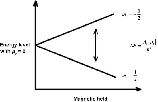
As shown in Figure 1, the splitting of energy levels due to the intrinsic dy-namics is similar to the Zeeman effect with the energy difference of
B
U g Bµ
∆ = .
Furthermore, if we also identify the intrinsic mass with the inertial mass of the electron,
µ
s =me, then the quantity As can be determined by all known physical quantities as3 2 2 s e ge B A m
= (48)
DOI: 10.4236/jmp.2019.1011091 1386 Journal of Modern Physics
Figure 1. Splitting of energy levels by intrinsic spin dynamics.
an external field. The dependence of quantity As on an external field is similar to the case of the inertial mass of an elementary particle that depends on the speed of the particle relative to a coordinate system formulated in Einstein’s
spe-cial relativity as 2 2
0 1
m m= −v c . It is interesting to mention here that in
fact we have shown in our work on the fluid state of an electromagnetic field that the electric field and the magnetic field can also be identified as velocity fields of a fluid [17].
5. A Generalised Formulation of Intrinsic Dynamics Using
Schrödinger Equation
From our discussion of the possibility to describe the spin angular momentum of a quantum particle as an intrinsic dynamics using the Schrödinger wave equa-tion, we may consider further extension by generalising the equation given in Equation (31) to a more general form so that it can be used to describe other in-trinsic dynamics that associate with a quantum particle, such as when a hydro-gen atom absorbs a photon, the photon may be considered to be correlated with the electron and accordingly behaves as an intrinsic dynamics of the electron. A general equation that include possible intrinsic dynamics associated with an elementary particle can be written as
(
)
( ) (
)
(
)
( ) (
)
(
)
2 2
1 1
2 2
1 1
1
1
, , , ,
2
, ,
, ,
, , , ,
, , 2
,
n n
N
s n s s n
s s
n
V r
V
E µ
µ =
− ∇ Ψ + Ψ
+ − ∇ Ψ + Ψ
= Ψ
∑
r r r r r r
r r r r r r r
r r r
(49)
DOI: 10.4236/jmp.2019.1011091 1387 Journal of Modern Physics that must be determined based on the characteristics of the motion under con-sideration. If all intrinsic dynamics are independent then Equation (49) can be separated into a system of equations as follows
( )
( ) ( )
( )
2 2
0
2µ ψ V ψ Eψ
− ∇ r + r r = r (50)
( )
( ) ( )
( )
22
1 1 1 1 1 1 1
1
2µ χ V χ Eχ
− ∇ r + r r = r (51)
( )
( ) ( )
( )
22
2 N N N N N N N
N
V E
χ χ χ
µ
− ∇ r + r r = r (52)
where E E1+ 2+ + EN =E. For example, if we assume that there are N1 two-dimensional and N2 three-dimensional intrinsic dynamics so that
1 2
N +N =N, and all intrinsic dynamics have the intrinsic potentials of the form
( )
s s s s
V r = A r then using Equations (8) and (42) we would obtain an expres-sion for the total energy spectrum as
(
)
2 2 2 2 1 2 2 2 22 21 1
0 2
1 , ,
4
2 2 1 2
2
N N
s s s s
s s
s s s
s s
A A
Zq E n n m
n n
n m
µ µ
µ
ε = =
= − − −
π + +
∑
∑
(53)As an example for the case of a three-dimensional intrinsic dynamics, let us consider an intrinsic dynamics that can be described as a spin dynamics of a photon when it is absorbed and then emitted from a hydrogen atom. If the pho-ton exhibits a three-dimensional intrinsic dynamics then we would obtain not only the normal three-dimensional Schrödinger wave equation for the hydrogen atom but also an intrinsic three-dimensional Schrödinger wave equation for the photon, similar to the system of equations given in Equations (32) and (33). In this case the total energy spectrum can be found as
(
)
2 2 2 2 22 20 1 , 4 2 2 s s s s A Zq
E n n
n n
µ µ
ε
= − π −
(54)
When the electron of the hydrogen atom at the energy level 𝑛𝑛 absorbs a photon and moves to a higher energy level n′, we may suggest that the photon also changes its energy levels from the level ns to the level ns′. We then obtain the new total energy level
(
)
( )
( )
2 2
2
2 2 2 2
0 1 , 4 2 2 s s s s A Zq
E n n
n n µ µ ε ′ ′ = − − ′ π ′
(55)
If we also assume that the energy difference E n n
(
′ ′ −, s)
E n n(
, s)
equals the Planck energy hν
then we obtain( )
( )
2 2
2
2 2 2 2 2 2
0
1 1 1 1
4
2 2 s s
s s
A Zq
h
n n n n
µ µ ν ε = − + − ′ ′
π
(56)
DOI: 10.4236/jmp.2019.1011091 1388 Journal of Modern Physics unless the photon is massive, i.e. µ ≠s 0, Equation (56) reduces to the familiar
energy spectrum of the hydrogen atom as shown in quantum mechanics.
6. Conclusion
We have shown in this work the possibility to formulate the spin dynamics asso-ciated with a quantum particle using Schrödinger equation in quantum me-chanics. Contrary to the general assumption that spin dynamics belongs to the domain of relativistic quantum mechanics that cannot be represented by a wa-vefunction, we have shown that spin dynamics can be formulated by a non-relativistic Schrödinger wave equation by considering possible intrinsic dy-namics conferred on quantum particles. Similar to the normal dydy-namics, intrin-sic dynamics can also be expressed in terms of Schrödinger wave equation by using intrinsic coordinates. Since intrinsic coordinates are independent to ex-ternal coordinates, the total Schrödinger wave equation can be separated into a system of Schrödinger wave equations each of which can be solved separately to obtain exact solutions and their corresponding eigenvalues for the energy. To il-lustrate, we have applied the formulations to the spin angular momentum for the electron of a hydrogen atom and shown that the quantum numbers asso-ciated with the spin angular momentum can take half-integral values, and these results can be used to explain the Stern-Gerlach experiment and other experi-ments that involve the electron spin resonance. Furthermore, we have also ap-plied the formulation to a possible spin dynamics associated with the radiation of a photon from a hydrogen atom.
Acknowledgements
We would like to thank the reviewers for their constructive comments and we would also like to thank Jane Gao of the administration of JMP for her editorial advice during the preparation of this work.
Conflicts of Interest
The author declares no conflicts of interest regarding the publication of this pa-per.
References
[1] Bransden, B.H. and Joachain, C.J. (1990) Physics of Atoms and Molecules. Long-man Scientific & Technical, New York.
[2] Pons, D.J., Pons, A.D. and Pons, A.J. (2019) Journal of Modern Physics, 10, 835-860. https://doi.org/10.4236/jmp.2019.107056
[3] Dirac, P.A.M. (1928) Proceedings of the Royal Society A: Mathematical, Physical and Engineering Sciences, 117, 610-624. https://doi.org/10.1098/rspa.1928.0023
[4] Ho, V.B. (2019) Journal of Modern Physics, 10, 1065-1082.
https://doi.org/10.4236/jmp.2019.109069
DOI: 10.4236/jmp.2019.1011091 1389 Journal of Modern Physics [6] Bransden, B.H. and Joachain, C.J. (1989) Introduction to Quantum Mechanics.
Longman Scientific & Technical, New York.
[7] Ho, V.B. (2018) Journal of Modern Physics, 9, 2402-2419.
https://doi.org/10.4236/jmp.2018.914154
[8] Newton, I. (1687) The Mathematical Principles of Natural Philosophy. Translated into English by Andrew Motte (1846).
[9] Einstein, A. (1952) The Principle of Relativity. Dover Publications, New York. [10] Ho, V.B. (2017) International Journal of Physics, 6, 105-115.
https://doi.org/10.12691/ijp-6-4-2
[11] Ho, V.B. (2018) Global Journal of Science Frontier Research, 18, 37-58. [12] Thaller, B. (1992) The Dirac Equation. Springer-Verlag, New York.
[13] Strauss, W.A. (1992) Partial Differential Equation. John Wiley & Sons, Inc., New York.
[14] Ho, V.B. (1994) Journal of Physics A: Mathematical and General, 27, 6237-6241.
https://doi.org/10.1088/0305-4470/27/18/031
[15] Ho, V.B. and Morgan, M.J. (1996) Journal of Physics A: Mathematical and General, 29, 1497-1510. https://doi.org/10.1088/0305-4470/29/7/019
[16] Ho, V.B. (1996) Geometrical and Topological Methods in Classical and Quantum Physics. PhD Thesis, Monash University, Clayton.
DOI: 10.4236/jmp.2019.1011091 1390 Journal of Modern Physics
Appendix
In this appendix we show in details the formulation of Maxwell field equations from the system of linear first order partial differential equations given in Equa-tion (10) of SecEqua-tion 3. The system of equaEqua-tions given in EquaEqua-tion (10) can be written the following matrix form
0 1 2 3 4
A A A A A J
t x y z ψ
∂ + ∂ + ∂ + ∂ =
∂ ∂ ∂ ∂
(1)
where
ψ
=(
ψ ψ ψ ψ ψ ψ
1, , , , ,2 3 4 5 6)
T,(
)
T 1, , ,0,0,02 3J= j j j and the matrices Ai
are given as follows
0 1
2 3
1 0 0 0 0 0 0 0 0 0 0 0 0 1 0 0 0 0 0 0 0 0 0 1 0 0 1 0 0 0 0 0 0 0 1 0
, ,
0 0 0 1 0 0 0 0 0 0 0 0 0 0 0 0 1 0 0 0 1 0 0 0 0 0 0 0 0 1 0 1 0 0 0 0 0 0 0 0 0 1 0 0 0 0 1 0 0 0 0 0 0 0 0 0 0
0 0 0 1 0 0 , 0 0 1 0 0 0 0 0 0 0 0 0 1 0 0 0 0 0
A A A A − − − − = = − − − = = − 4
1 0 0 0 0 0 0 0 0
, 0 1 0 0 0 0 1 0 0 0 0 0 0 0 0 0 0 0 0 0 0 0 0
0 0 0 0 0 0 0 0 0 0 0 0 0 0 0 0 0 0 0 0 0 0 0 0 0 0 0 0 A µ µ µ − = (2)
The system of equations given in Equation (1) becomes
6 5
1
1 j
t y z
ψ ψ
ψ ∂ ∂ µ
∂
− + − =
∂ ∂ ∂ (3)
6
2 4
2 j
t z x
ψ
ψ ψ ∂ µ
∂ ∂
− + − =
∂ ∂ ∂ (4)
3 5 4
3 j
t x y
ψ ψ ψ µ
∂ ∂ ∂
− + − =
∂ ∂ ∂ (5)
3
4 2 0
t y z
ψ
ψ ∂ ψ
∂ ∂
+ − =
∂ ∂ ∂ (6)
5 1 3 0
t z x
ψ ψ ψ
∂ ∂ ∂
+ − =
∂ ∂ ∂ (7)
6 2 1 0
t x y
ψ ψ ψ
∂ ∂ ∂
+ − =
DOI: 10.4236/jmp.2019.1011091 1391 Journal of Modern Physics Using the identification E=
(
ψ ψ ψ
1, ,2 3)
and B=(
ψ ψ ψ
4, ,5 6)
, the above system of equations can be rewritten in the familiar form given in classical elec-trodynamics ase
ρ
⋅ =E
∇ (9)
0
⋅ =B
∇ (10)
0
t ∂
× + =
∂ B E
∇ (11)
e
t
µ∂ µ
× − =
∂ E
B j
∇ (12)
where the charge density ρe and the current density je satisfy the conserva-tion law
0
e e t
ρ ∂
⋅ + =
∂ j
∇ (13)
From the matrices Ai given in Equation (2) we obtain
2 2
0 1
1 0 0 0 0 0 0 0 0 0 0 0 0 1 0 0 0 0 0 1 0 0 0 0 0 0 1 0 0 0 0 0 1 0 0 0
, ,
0 0 0 1 0 0 0 0 0 0 0 0 0 0 0 0 1 0 0 0 0 0 1 0 0 0 0 0 0 1 0 0 0 0 0 1
A A
−
−
= =
−
−
2 2
2 3
1 0 0 0 0 0 1 0 0 0 0 0 0 0 0 0 0 0 0 1 0 0 0 0 0 0 1 0 0 0 0 0 0 0 0 0
, ,
0 0 0 1 0 0 0 0 0 1 0 0 0 0 0 0 0 0 0 0 0 0 1 0 0 0 0 0 0 1 0 0 0 0 0 0
A A
− −
−
−
= − = −
−
−
2
2
2 2
4 1 2 2 1
0 1 0 0 0 0 0 0 0 0 0
1 0 0 0 0 0
0 0 0 0 0
0 0 0 0 0 0
0 0 0 0 0
,
0 0 0 0 1 0 0 0 0 0 0 0
0 0 0 1 0 0 0 0 0 0 0 0
0 0 0 0 0 0 0 0 0 0 0 0
A A A A A
µ
µ
µ
= + =
1 3 3 1 2 3 3 2
0 0 1 0 0 0 0 0 0 0 0 0 0 0 0 0 0 0 0 0 1 0 0 0
1 0 0 0 0 0 0 1 0 0 0 0
,
0 0 0 0 0 1 0 0 0 0 0 0 0 0 0 0 0 0 0 0 0 0 0 1 0 0 0 1 0 0 0 0 0 0 1 0
A A A A A A A A
+ = + =
0 i i 0 0 for 1,2,3
DOI: 10.4236/jmp.2019.1011091 1392 Journal of Modern Physics Now, if we apply the differential operator
(
A0∂ ∂ + ∂ ∂ +t A1 x A2∂ ∂ +y A3∂ ∂z)
to Equation (1) then we arrive at2 2
2 2
2
1 0 0 0 0 0 0 0 0 0 0 0 0 1 0 0 0 0 0 1 0 0 0 0 0 0 1 0 0 0 0 0 1 0 0 0 0 0 0 1 0 0 0 0 0 0 0 0 0 0 0 0 1 0 0 0 0 0 1 0 0 0 0 0 0 1 0 0 0 0 0 1
1 0 0 0 0 0 0 0 0 0 0 0 0 0 1 0 0 0 0 0 0 1 0 0 0 0 0 0 0 0 0 0 0 0 0 1
t x − ∂ + − ∂ ∂ ∂ − − − − ∂ + − − 2 2 2 2 2
1 0 0 0 0 0 0 1 0 0 0 0 0 0 0 0 0 0 0 0 0 1 0 0 0 0 0 0 1 0 0 0 0 0 0 0 0 1 0 0 0 0 0 0 1 0 0 0
1 0 0 0 0 0 0 0 0 0 0 0 0 0 0 0 0 0 1 0 0 0 0 0 0 0 0 0 1 0 0 0 0 0 0 1 0 0 0 1 0 0 0 0 0 0 0 0 0 0 0 0 0 0 0 0 0 1 0 0 0 0 0 0
y z
x y x z
− − ∂ + − ∂ ∂ − ∂ ∂ + + ∂ ∂ ∂ ∂ + 2
0 0 0 0 0 0 0
0 0 1 0 0 0 0 0 0 0 0
0 1 0 0 0 0 0 0 0 0 0
0 0 0 0 0 0 0 0 0 0 0 0 0 0 0 0 0 1 0 0 0 0 0 0 0 0 0 0 1 0 0 0 0 0 0 0
J
y z t
µ µ µ ψ ∂ ∂ = − ∂ ∂ ∂ (15)
From Equation (15), we obtain the following system of equations for the elec-tric field E=
(
E E Ex, ,y z)
=(
ψ ψ ψ
1, ,2 3)
2 2 2
3
1 1 1 2 1
2 2 2
j
x y z t
t y z
ψ
ψ ψ ψ ψ ∂ µ
∂ −∂ −∂ + ∂ ∂ + = − ∂
∂ ∂ ∂ ∂
∂ ∂ ∂ (16)
2 2 2
3
2 2 2 1 2
2 2 2
j
y x z t
t x z
ψ
ψ ψ ψ ψ
µ ∂
∂ −∂ −∂ + ∂ ∂ + = − ∂
∂ ∂ ∂ ∂
∂ ∂ ∂ (17)
2 2 2
3 3 3 1 2 3
2 2 2
j
z x y t
t x y
ψ ψ ψ ψ ψ µ
∂ −∂ −∂ + ∂ ∂ +∂ = − ∂
∂ ∂ ∂ ∂
∂ ∂ ∂ (18)
If the electric field also satisfies Gauss’s law
3
1 2 e
x y z
ψ ρ
ψ ψ ∂
∂ ∂
⋅ = + + =
∂ ∂ ∂
E
∇ (19)
then we obtain the following relations
2 3
2 1 1
2
e e
x y z x x x x
ψ ρ ρ
ψ ∂ ψ ψ
∂ ∂ ∂
∂ + = ∂ − = − + ∂
DOI: 10.4236/jmp.2019.1011091 1393 Journal of Modern Physics 2
3
1 2 2
2
e e
y x z y y y y
ψ ρ ρ
ψ ∂ ψ ψ
∂ ∂ ∂
∂ + = ∂ − = − + ∂
∂ ∂ ∂ ∂ ∂ ∂ ∂ (21)
2
3 3
1 2
2
e e
z x y z z z z
ρ ψ ψ ρ
ψ ψ ∂ ∂
∂ ∂
∂ + = ∂ − = − + ∂
∂ ∂ ∂ ∂ ∂ ∂ ∂ (22)
From Equations (16-18) together with relations given in Equations (20-22), we obtain, in vector form, the wave equation for the electric field as
2 2
2 e te
t
ρ µ∂
∂ − ∇ = ∇ −
∂
∂
J
E E
(23)
where Je =
(
j j j1, ,2 3)
. Similarly for the magnetic field(
B B Bx, ,y z)
(
ψ ψ ψ
4, ,5 6)
= =
B we obtain the following equations and relations
2 2 2
5 6
4 4 4
2 2 2 x y z 0
t y z
ψ ψ
ψ ψ ψ ∂ ∂
∂ −∂ −∂ + ∂ + =
∂ ∂ ∂
∂ ∂ ∂ (24)
2 2 2
5 5 5 4 6
2 2 2 y x z 0
t x z
ψ ψ ψ ψ ψ
∂ −∂ −∂ + ∂ ∂ +∂ =
∂ ∂ ∂
∂ ∂ ∂ (25)
2 2 2
6 6 6 4 5
2 2 2 z x y 0
t x y
ψ ψ ψ ψ ψ
∂ −∂ −∂ + ∂ ∂ +∂ =
∂ ∂ ∂
∂ ∂ ∂ (26)
5 6
4 0
x y z
ψ ψ
ψ ∂ ∂
∂
⋅ = + + =
∂ ∂ ∂
B
∇ (27)
2
5 6 4
2
x y z x
ψ ψ ψ
∂ ∂
∂
∂ + = −
∂ ∂ ∂ ∂ (28)
2
6 5
4
2
y x z y
ψ ψ
ψ ∂ ∂
∂
∂ + = −
∂ ∂ ∂ ∂ (29)
2
5 6
4
2
z x y z
ψ ψ
ψ ∂ ∂
∂
∂ + = −
∂ ∂ ∂ ∂ (30)
2 2
2 0
t
∂ − ∇ =
∂