A Novel Method for Remotely Sensed Hyperspectral Image Classification Based on Convolutional Neural Network

ISSN: 1816-949X

© Medwell Journals, 2020

A Novel Method for Remotely Sensed Hyperspectral Image Classification

Based on Convolutional Neural Network

1

_{B.R. Shivakumar and}

2

_{J. Prakash}

1

_{Department of Information Science and Engineering, Bangalore Institute of Technology,}

Visvesvaraya Technological University, K.R. Road, V.V. Puram,

Belagavi, Bengaluru, India

2

_{Department of Information Science and Engineering, Bangalore Institute of Technology,}

K.R. Road, V.V. Puram, Bengaluru, India

Abstract: The Hyperspectral Images (HSI) acquired by remote sensors are characterized by hundreds of

contiguous channels with high spectral resolution. Hyperspectral image classification is the process of assigning land cover classes to pixels. Classifying remotely sensed data is a challenge because many factors such as complexity of landscape, image processing and classification approaches affect the success of classification. Convolutional Neural Networks (CNN) are gaining attention due to their capability to automatically discover relevant relative features in image classification problems. The proposed approach employs totally eight layers in which four convolutional layers, two pooling layers and two Fully Connected Network (FCN) hidden layers to extract features from hyperspectral images. This method is able to extract the features invariably for their location and distortion which leads to better classification accuracy. By extracting both spatial and spectral information, the performance of the model is a promising one for high dimensional HSI with few available training data. This method has been applied to University of Pavia and Indian pines datasets. The resultant of the model demonstrates very good classification accuracy within limited number of training epochs.

Key words: Convolution layer, convolutional neural networks, deep learning, fully connected network,

hyperspectral image classification, land cover classification

INTRODUCTION

Remotely sensed hyperspectral images are very much essential to meet the ever growing demand of satellite images with spectral, spatial, temporal and radiometric high resolutions. HSI captures the reflected radiation from the earth surface as series of narrow and contiguous wavelength bands. Compared to multispectral images HSI provides more rich spectral information. Images represented as three dimensional cube with respect to a scene in which x and y-axis represents spatial data and z-axis represents, the spectral data for the same scene. The richer spectral information presents, the detailed characteristics and uniqueness of the materials (Lu and Weng, 2007).

The motivation of classification is to convert continuous data into categorical information classes, describing the landscape. The classified image can be used for decision making for effective management of natural resources by linking each pixel to one or more user defined labels like vegetation, water, built up etc. Due to high dimensionality of the pixel, heterogeneity, noise, spatial and spectral redundancy, atmospheric and geometric distortions, the characteristics of the image,

lead to nonlinear feature relations. All these non-linear factors with very few labelled classes make HSI classification a challenging problem. The major steps of image classification may include determination of a suitable classification system, selection of training samples, image pre-processing, feature extraction, selection of suitable classification approaches, post classification processing and accuracy assessment. The several factors such as the spectral and spatial resolution, sources of images, classification methods affects the accuracy of the classification. Various classification techniques has their own merits and demerits in each situations. Based on pixel information, images can be classified as per-pixel, sub-pixel, per-field, knowledge based, contextual and multiple classifiers. Per-pixel classifiers may be parametric or non-parametric. Based on the use of training samples, images can be classified using supervised or unsupervised or semi supervised classification methods (Kamavisdar et al., 2013).

In this study, HSI classification is carried out using CNN method which is a powerful feature learning model. It is built using stacked convolution, pooling and Fully Connected Network (FCN) layers. It learns both the hierarchical, discriminative features which helps in better Corresponding Author: B.R. Shivakumar, Department of Information Science and Engineering,

classification over hard-wired classification model. The model is adaptive, trains both feature extractor and classifier together in supervised mode. Therefore, it is most suitable for HSI classification task which is characterized by rich spectral and spatial domain information.

Literature review: The high number of features

encountered in remote sensing HSI classification tasks from use of simple statistical classifiers, commonly employed in multispectral image classification are ineffective. Therefore, more sophisticated classifiers must be used to exploit the rich spectral information offered by HSI. In this way, different techniques have been proposed from the field of pattern recognition and artificial intelligence for handling hyperspectral data.

The broadly used Principle Component Analysis (PCA), Independent Component Analysis (ICA) focuses on spectral dimensionality reduction based classification techniques which transforms the data into new domain to extract potentially better features (Villa et al., 2011; Licciardi et al., 2012). Support Vector Machines (SVMs) is a binary classifier which assigns a test sample to any one of the class and it is a non-parametric statistical learning method. It is investigated that this technique is applied without the necessity of feature reduction process and it works better with less number of training samples (Mountrakis et al., 2011; Melgani and Bruzzone, 2004). The Extreme Learning Machine (ELM) is a single hidden layer feed-forward neural network which is computationally efficient pattern classification approach. The weights of input to hidden layer are randomly applied and hidden to output layer weights are leant while training which results in poor training o no solution. This weaker learner is tied with another weak leaner to build strong learner. ELM used for classification of HSI is a challenge due to its high spectral data (Samat et al., 2014). Yicong Zhou et al. (2015) proposed, two spatial-spectral composite kernel ELM classification methods in which the spatial or spectral kernel has activation function, Gaussian based kernel, respectively for HSI classification. But the small architecture of ELM has limited distinguishing power.

Active learning can successfully reduce labelling tasks for remote sensing image classification. The active learning procedure is based on the uncertainty sampling strategy and a deep neural network. Stacked auto-encoders trained on redundant spatial and spectral features and a few labelled training samples are used to initialize a deep neural network. Uncertainty for a given sample is measured by the difference between the largest two class outputs of the neural network. The less difference there is the more uncertainty the sample has. Batch of samples with most uncertainty will be selected

after label query and added into the training set. Then the neural network is retrained and such active batch selection will iterate until the budget (the upper limit of label queries) is reached (Licciardi et al., 2012). Initially, k-means clustering is employed for unsupervised learning and knowledge discovery for HSI. Training data is prepared for neural network and tested with different scenes of spatial and spectral variations. The performance of proposed ensemble classifier is analyzed in terms of overall and average accuracy. Ensemble classifier is designed by employing support vector machine and neural network to further improve the accuracy (Rudrapal and Subhedar, 2016). Granular Neural Network (GNN) in combination with the granular representation of information using linguistic terms is one such system. GNN takes the fuzzified input information and processes them with neural network architecture where the network structure is transparent enough to interpret the processing steps. Further, knowledge encoding has been considered as one of the principal elements of intelligent decision-making systems. This study proposes a new model of knowledge-encoded GNNs for land cover classification of HSI images. Knowledge encoding is done using Neighbourhood Rough Sets (NRSs) that explore the local/contextual information. The encoded knowledge using NRS is obtained in the form of dependency rules with respect to the output class labels of land covers and these rules determine appropriate number of hidden nodes of GNNs. The dependency factors obtained during rule generation are used for initializing the connecting weights of GNNs. NRS is also used here in the selection of a subset of features for reducing the burden of high-dimensional fuzzy-granulated feature space of HSI image (Meher, 2015).

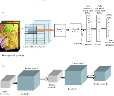
Fig. 1: (a) Architecture for proposed HSI classification CNN Model and (b) A stage representing a sequence of Convolution1-Convolution2-Maxpooling stages (C-C-M)

MATERIALS AND METHODS

This study describes the architecture and the algorithm of the proposed methodology for classification HSI using CNN technique. The architectural network of the proposed method is presented as shown in Fig.1a and b.

In this study the architecture of the model and algorithm for training and testing for classification of HSI using CNN method is explained. CNN is feed-forward neural network which is a combination of convolution layer, pooling and FCN layers. This model is based on the principle of deep neural network architecture which learns spectral-spatial features and gives better performance in classification. The architecture diagram, mainly consists of three cascaded steps which are patch extraction, convolution and max pooling, Fully Connected Layer (FCN) as shown in Fig. 1a. The output of the model is class label O_i for corresponding pixel Pi. The

entire network is trained by back propagating the error. The filter kernels of convolution layers and link weights of FCN are updated depend upon the error.

In patch extraction step, a pixel Pi represented by a

patch of the input HSI with its neighborhood of the size R_p×C_p (Spatial adjacent features) along N_b bands

(Spectral features) is extracted. The successive pixel representing patches, contains overlapping window of the neighborhood patches. Then the patch representing a pixel presented to first convolution layer of stage-I which is consists of two cascaded convolution layers and a max pooling layer as shown in Fig. 1b.

Inspired by the biological visual systems, CNN architecture is evolved for computer vision applications. In the human vision system, there are two types of cells in the visual cortex such as simple cells and complex cells. The simple cells determines local features, specifically edge-like patterns whereas complex cells aggregates the outputs of neighborhood simple cells. The complex cells have bigger receptive fields relative to simple cells and they are invariant to local features. Similarly, the architecture of CNN has two features, local connections and shared weights. The local connection extracts local correlation whereas shared weight facilitate in detecting features, irrespective of their positions in the field of view. Due to the shared weights, the number of trainable parameters get reduced. The combination of both the features helps in better generalization of the model.

In this case, a patch of input image having Rp rows,

C_p columns and N_b bands (R_p×C_p×N_b) is convolved by the weights which is nothing but trainable filter kernels of the Filters

FR×FC×F1 RP×CP×F1

RP×CP×F2 Filters

FR×FC×F2

(RP/2)×(CP/2)×F2 Feature maps 1

Feature maps 2 (b)

(a)

Hyperspectral input image

A patch of Rp×Cp×Nb size

Stage-I C-C-M

Stage-II C-C-M

Flattening

M nodes N nodes

O Nodes Number of class labels Fully

connected hidden layer

FC-h1

Fully connected hidden layer

FC-h2

[image:3.612.115.501.82.408.2]

size FR×FC×Nb across the entire patch in that layer. At any

instant, the kernel weights (F_R×F_C) are convolved with a window which is smaller than the image and extracts features local to the window. But the same kernel weights are used to extract similar features across the whole image, hence, sharing of the kernel weights for the whole image. Typically, the filter size may be 3×3 or 5×5 and it is convolved over the image of 16×16. The resultant feature maps of size N_b aresummed up to produce, single Rp×Cp sized feature map corresponding a given filter.

Similarly, F1 number of feature maps are produced using

F1×Nb number of kernels for the same patch each

representing particularly specific feature. The resultant of the convolution as shown in Eq. 1, produces a activation layer. Then, these activation layers are converted into non linear by applying Rectified Linear Unit (ReLU) as in Eq. 2. The output of the activation function is F1 number

of feature maps of the size Rp×Cp. Typically, F1= 400 in

the first convolution of stage-I layer:

(1)





1 1 -l 1

i i, j i i j

A =



f w *A +b

Where: Al

i : The activation of the ith feature map in lth layer

Ai

l-1_{: The activation in ith feature map in (l-1)th layer}

that is previous layer wl

i, j: The convolution kernel (Filter kernel) for Ai l-1

bl _{: Bias}

* : Convolution operator

(2)

 

1



1



i i

Fi = f A = max 0, A

where, Fi is feature map of ith layer. The number of filter kernels, filter size, the stride and amount of zero padding are hyper parameters in CNN which are tuned to obtain better performance and this is essential for the type of input image, number of class labels, computing speed and available computing resources.

The depth of feature maps corresponds to the number of filters at each convolution layer, represents various oriented edges, blobs of colour for the same region of input image. The large number of feature maps leads to more requirement of memory and computation time. Hence, this parameter has to be balanced for a given problem. The stride refers to the number sliding pixels after a convolution operation of filter over a window of input image. Suppose, the stride is one, the filter moves one pixel at a time and for stride value of two, the filter jumps two pixels at a time. More the number of strides, the output will reduce across spatial dimensions. To cover the border pixels of the images, it is essential to pad the image with zero, therefore, output feature map spatial size will be retained as that of the input image.

In stage-I, F₁ number of features obtained by first convolution layer becomes input to second convolution layer. In the second layer also convolution and activation

functions are applied on Rp×Cp×F1 sized input as in Eq. 1

and 2. The output produced at second convolution layer with the depth of F2 feature maps of the spatial size Rp×Cp

is fed to max pooling layer. Through this operation, the feature are made invariant from, the location and distortion. This layer reduces the spatial size of the feature maps by retaining the depth and concise the features. Therefore, the computation burden of subsequent layers is reduced. The max pooling operation, partitions the input feature map into a set of non overlapping windows. Then, the maximum value is chosen from the local pool window of the feature map as in Eq. 3. In case of the window size 2×2 then the output of this layer has the size (Rp/2)×(Cp/2)×F2:

(3)

 



nxn



j i

v = max v u n, n

where, vj is maximum in the neighbourhood of N×N

window, u (n, n) is the window function to the patch of feature map, vi is the input window at location i in the

feature map.

The stage-II operations are similar to the stage-I, except the depth of the feature maps. The output of the stage-II has the spatial size (Rp/4)×(Cp/4) and feature

maps depth as F4.In the first layer of stage-I, the feature

map may contain low level features like edge of particular orientation, lines etc. The following convolution, pooling layers helps to detect higher level features like curves, textures. Eventually, the feature maps may contain the parts, patterns present in the scene that is entire visual concept. The main advantage of increasing the layers is to increase the visual hierarchy of concepts with smaller representation. To classify the feature detected in convolution layer, FCN is used as final stage in CNN. The stage-II output F4 feature maps of the size

(R_p/4)×(C_p/4)×F₄ are converted to 1-D vector to feed to FCN. This layer is a multi-layer perceptron neural network which connects all nodes of one layer to all nodes of next layer associated with activation function. The FCN is comprising of one input layer which has same number of nodes as that of output of max pooling layer, followed by two hidden layers h1 and h2 with M and

N number of nodes, respectively. The computational procedure is presented for hidden layer h1 of FCN as in

Eq. 4 and 5:

(4)





linet h1 hl l

h = f W , b for all M nodes

in h layer

Where:

(5)

L linet hl j = 1

h = b +



WjCj for all M nodes

Where:

Activation function, Rectified Linear Unit (ReLU) is used to threshold the activation at zero as in Eq. 6:

(6)









li linet linet

h = f h = max 0, h

Similarly, the net and activated output values for N nodes in h2 layer is computed same as in hidden layer

h₁. Finally, the output of h₂ layer is terminated at output layer consisting of O number of nodes which represents the desired number of class labels to be determined. The input pixel is classified at this last layer by using softmax as its activation function. The classification of an input pixel is computed based on the conditional probabilities of the O output classes as in Eq. 7. Conditional probability for O classes, Pc = (Pc1, Pc2, Pc3, PcO). For

each class, the probability distribution (Chen et al., 2016) computed as:

(7)

yi i 0 yi

i = 1

e P =

e



where, yi = (y1, y2, y3, ..., yO) is the input to

softmax activation function at the output layer. The back-propagation algorithm is used to minimize the error between the desired and actual output. The error is calculated by various cost or loss functions. In training process, the derivative of the error value is back-propagated, so that, the link weights in FCN and kernel weights are updated to the optimal values. In this implementation, cross entropy loss function has been adopted. Suppose, O is the number of class labels then {P_i, T_i} for i = 1 to N, training set in which P_i is the input patch representing a pixel and Ti is a corresponding target

class. The loss function (Yang et al., 2016) for classification is given in Eq. 8:

(8)

 

N 0



 



 

n = 1 k = 1 k

1

C = - f k = T n log P n

N



 

Where:

N : The number of training patches

T (n) : A ground truth label of the nth training sample Pk (n) : The kth element

P (n) : Which is the conditional probability of assigning kth class to the nth sample

The indicative function f (k = T (n)) is 1 if the condition is met, else it is 0. Φ denotes the set of convolutional kernels and bias values.

The following algorithm presents the working procedure to obtain, optimal model for HSI classification. This algorithm has several steps to work with this model such as model building, dataset preparation, model parameter initialization, fine tuning of the model, training and testing of the model to accomplish the task.

Algorithm for CNN training and testing for HSI classification: The steps for training and testing of HSI classification are listed as below.

Step 1: Construction of the network:

i. Build the CNN Model in the sequence as {Convolution layer-convolution layer-maxpool layer-layer-convolution layer-layer-convolution layer-maxpool layer-hidden layer 1-hidden layer 2-output layer} as shown in Fig. 1

ii. Set the number of filters and nodes as {F1-F2-F3-F4-M-N-O}. Set maxpool layer window size = 2×2

iii. Set the activation function as ReLU as in Eq. 2 to all convolution layer and hidden layer. Set softmax activation function to output layer in FCN as in Eq. 7

Step 2: Preparation of the dataset:

i. Normalize all the pixel value of the image that is scale down the pixel value (0-255) to (0.0-1.0)

ii. Read a pixel, equally surrounded by Rp×Cp pixels across Nb number of bands that is a patch image of the size Rp×Cp×Nb. Read the ground truth label for the corresponding input pixel and set it as a target class. Repeat the same process for all the R×C pixels of the input HSI

iii. Shuffle the patches along with their target class

iv. Split the R×C number of pixels in the ratio of 7.5:2.5 in which 75% of pixels will be used for training, 25% for testing purpose

Step 3: Initialization of the model:

i. Initialize all filter kernels, FCN weights and biases to random numbers

ii. Initialize the learning rate α to 10-3_{, maximum number of epochs,} training batches, batch size, stride and zero padding

iii. Set the loss function as shown in Eq. 8

Step 4: Training: i. For each epoch, Do

ii. Input the batch of patches {batch, patches} to the network and compute the Oi of every unit i in the output layer

iii. For each Oi, compute conditional probability Pi as in Eq. 7 iv. For each output node Oi, compute loss function as in Eq. 8 v. Update each network weight by w = w+Δw where Δw = αδp,

α6learning rate, δ6rate of change of error, p6input to that node or kernel

vi. Back propagate the loss until it reaches the first convolution layer and update the weights of kernels, link weights of FCN and biases vii. Go to step 4 (ii) until all the batches completed

viii. Stop when the number of predetermined epochs completed

Step 5: Testing:

i. Consider testing sample patches and feed them to the network as described in step 4. The weights of the network should not be updated

ii. The actual output class is compared with the ground truth target class. The classification errors are calculated

iii. Suppose the accuracy is reached to the desired level, go to step 7

Step 6: Fine tuning of the model:

i. Suppose the accuracy is not up to the expected value, modify the hyper parameters such as learning rate, cost function, number of filters in convolution layers, strides, maxpooling window size, number of hidden layers, number of nodes in hidden layers, patch size, combination of convolution and maxpooling layers and so on. Go to step 1 and repeat the training

Step 7: Readiness of the model:

When the model is ready with the optimized weights can be used for application

RESULTS AND DISCUSSION

Experimental results and analysis: In this study, the

details of experiment setup the dataset specification, the results obtained and analysis of the data and results are discussed.

Experiment set up and datasets: In this study, the

experiments conducted using proposed HSI classification method is presented. Initially, the CNN Model is built with the convolution layers and fully connected layers. In this method, the patch of an image of the size of R_p×C_p×N_b is extracted from the input HSI and fed to CNN network. In this experiment, patch size considered are 5×5×B, 7×7×B, 9×9×B where B is the size of the number of bands in HSI. In this experiment, the filter sizes selected as 3×3×Fn for all the convolution layers where Fn

is the size of feature maps. In the stage-I, the values of F₁ and F₂ are 500 and 400, respectively and in stage-II, F₁ and F2 are chosen as 200 and 100, respectively. The

maxpooling operation is carried out to reduce the spatial size of the feature maps, after the successful two convolutions in both the stages of layer 1 and 2. After this operation the spatial size of feature maps get halved. The final feature map obtained at the end of layer 2 operation is flattened to one dimensional vector. The 1-D vector is fed to FCN. In this experiment at Fully Connected hidden layer (FC-h1), M = 200 and at second hidden layer FC-h2,

N = 100. The output layer has the number of nodes equal to the number of class labels that is O = 16 in the case Indian pines dataset and O = 9 for Pavia university dataset. The activation functions employed in hidden layers and output layer are ReLU and sigmoidal functions, respectively.

The training data is used for updating convolution filter values and weights in the fully connected network. The testing data samples are used for evaluating the proposed model. The learning rate has been experimented from 0.1-10-4 _{for better accuracy}

. The size of the feature

maps and number of nodes in the hidden layer of FCN are varied and tested to improve the performance of the model.

To experiment, two standard hyperspectral images of different characteristics such as spectral and spatial resolution, land cover, area size are considered. The first one is AVIRIS hyperspectral image of Indian pines (Baumgardner et al., 2015) and the second image used is of Pavia University in Northern Italy.

[image:6.612.314.540.103.383.2]

In this proposed methodology, a patch is considered as a training example which represents a pixel surrounded by its neighborhood pixels. Approximately, 10000 samples are shuffled and divided into training set and testing set in the ratio of 7.5:2.5, respectively. The performance of the proposed model is assessed using overall accuracy (Provost et al., 1998):

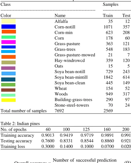
Table 1: Land cover classes for Indian pines dataset

Class Samples

--- ---Color Name Train Test Alfalfa 35 12 Corn-notill 1071 357 Corn-min 623 208 Corn 178 60 Grass-pasture 363 121 Grass-trees 548 183 Grass-pasture-mowed 21 7 Hay-windrowcd 359 120

Oats 15 5

Soya bean-notill 729 243 Soya bean-mintill 1842 614 Soya bean-clean 445 149 Wheat 154 52 Woods 949 317 Building-grass-trees 290 97 Stone-steel-towers 70 24 Total number of samples 7692 2569

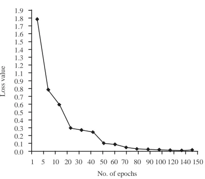
Table 2: Indian pines

No. of epochs 60 100 125 160 200 Training accuracy 0.9013 0.9419 0.9719 0.9891 0.991 Testing accuracy 0.7600 0.8331 0.8544 0.8860 0.921 Training loss 0.3000 0.1400 0.1000 0.0700 0.020

(9)

Number of successful prediction Overall accuracy =

Total number of prediction

Classification of Indian pines scene: The Indian pines

image (Baumgardner et al., 2015) has spatial resolution of 20 m2 _{per pixel and spectral resolution of 224 spectral}

bands in the range of 400-2500 nm which covers visible and infrared region. This image scene has 3/4th area of agricultural land and some part as forest vegetation. Also, there are buildings, railway tracks and highways in the image scene. The ground truth is available for 16 classes such as fields of corn, wheat, soybean, oats, stone-steel structures and other objects as shown in Table 1. The total size of the image is 145×145 pixels which covers the area of 2×2 miles.

Lo

ss

v

alu

es

1 10 25 50 75 100 125 150 175 200

No. of epochs 3.0

2.8 2.6 2.4 2.2 2.0 1.8 1.6 1.4 1.2 1.0 0.8 0.6 0.4 0.2 0.0

1.2

1.0

0.8

0.6

0.4

0.2

0.0

60 100 125 160 200

No. of epochs

A

cc

u

ra

cy

[image:7.612.111.493.97.460.2]

Training accuracy Testing accuracy

[image:7.612.329.529.507.645.2]

Fig. 2: Indian pines ground truth and classified images: (a) Indian pines ground truth, (b) Accuracy = 0.76 and (c) Accuracy = 0.92

Fig. 3: The loss of training dataset of Indian pines versus number of epochs

of ground truth image and the predicted image has been carried out at the interval of every 25 epochs. For better understanding of the effectiveness of accuracy, the ground

Fig. 4: The over all accuracy of Indian pies dataset versus number of epochs

truth and predicted images are presented as shown in Fig. 2b through Fig. 2c for the testing accuracies of 76% and 92%, respectively (Fig. 2-4).

(b) (a)

(c)

0 20 40 60 80 100 120 140 0

20

40

60

80

100

120

140

Va

lue

s

Variables 0

20

40

60

80

100

120

140

0

20

40

60

80

100

120

140

Va

lue

s

Va

lue

[image:7.612.89.282.510.644.2]

J. Eng. Applied Sci., 15 (1): 13-22, 2020 1.01 1.00 0.99 0.98 0.97 0.96 0.95 0.94 0.93 0.92

50 75 100 130 155

No. of epochs

[image:8.612.113.510.93.334.2]

A cc u rac y Training accuracy Testing accuracy

Fig. 5: Pavia University ground truth and classified images: (a) Pavia ground truth (b) Accuracy = 0.9235 and (c) Accuracy = 0.975

It is clearly shows that the predicted image of 92% has less number of misclassification compared to 76%. Through these evident, the proposed algorithm is better for HSI classification. The loss or the error value across various epochs are observed as shown in Table 2. The loss is reducing drastically till the 60th epoch. Afterwards, the error is gradually reducing and it is observed after 200 epoch, it is stuck at minimum value of 0.05 as shown in Fig. 3. The overall accuracy is achieved through this proposed model for training is 99% and testing accuracy 92%.

Classification of Pavia University scene: This image is

captured from the Reflective Optics System Imaging Spectrometer (ROSIS) sensors and have spatial resolution of 1 .2 m2 _{in the spectral range of 430-860 nm with}

[image:8.612.328.528.383.488.2]

103 spectral bands. The Pavia University image has the size of 610×340 pixels. The image scene has the building, roads covered with different materials like bitumen, asphalt, gravel, land cover by meadows, bare soil, metal sheets structures, trees as shown in Table 3 which covers 9 classes. The Pavia University image is applied to the proposed model of HSI classifier to study the performance of the model for high resolution images. In this case also the overall accuracy of the predicted image computed in both training and testing phase as tabulated in Table 4 and Fig. 6. For the visual evidence Fig. 5 (a) through (c) is presented with ground truth of Pavia University and predicted images at the accuracy of 92.35 and 97.5% testing accuracy.

[image:8.612.317.541.532.654.2]

Fig. 6: The overall accuracy of Pavia dataset versus number of epochs

Table 3: Land cover classes for Pavia University

Class Samples

--- ---Color Name Train Test

Asphalt 4974 1658 Meadows 13987 4663 Gravel 1575 525 Trees 2298 766 Metal sheets 1009 337 Bare soil 3772 1258 Bitumen 998 333 Bricks 2762 921 Shadow 711 237 Total 32082 10698

The model is converging faster when compared to Pavia dataset due to its high resolution. It is also observed that the testing accuracy is very much close to training accuracy. The loss computed at various epochs are presented in Table 4 and its graph in Fig. 7. The loss is 0.1 at 50th epoch and it is reduced to small as 0.01 at (a)

0 100 Varia 0 100 200 300 400 500 600

200 300 ables

Va

lue

s

(b)

0 50 10 0 100 200 300 400 500 600 Variables 00 150 200 250 3

Va lue s 0 100 200 300 400 500 600 300 (c)

0 50 100 150 Varia

1.9 1.8 1.7 1.6 1.5 1.4 1.3 1.2 1.1 0.9 0.8 0.7 0.6 0.5 0.4 0.3 0.2 0.1 0.0

L

os

s v

a

lu

e

1 5 10 20 30 40 50 60 70 80 90 100 120 140 150

[image:9.612.84.284.88.263.2]

No. of epochs

Fig. 7: The loss of training dataset of Pavia University versus number of epochs

Table 4: Pavia University

No. of epochs 50 75 100 130 155 Training accuracy 0.9637 0.9872 0.9968 0.9975 0.9988 Testing accuracy 0.9510 0.9597 0.9715 0.9750 0.9752 Training loss 0.1100 0.0400 0.0200 0.0100 0.0080

120th epoch. Since, the applied image dataset is very high resolution and more distinguishable in the object spacing in the scene has made the model to reach the accuracy at lower number of epoch training. This model outperformed in this scene with respect to testing accuracy and convergence time such as 97.52% at 115 epochs.

CONCLUSION

In this study, a new eight layer HSI classification model based on deep convolutional neural network is proposed. The proposed CNN Model takes the input of both spectral and spatial data as a patch by considering the neighborhood of the pixel of interest. The experimental result shows that the proposed method improves the overall classification accuracy of the model for small number of epochs. The experiment has been conducted for different spatial and spectral resolution images. The results are verified for the effectiveness of the method by computing the classification accuracy for different number of epochs. The classification into the required output classes was successfully performed. The testing accuracy of 97% is achieved through this experiment. This classification is used to classify all pixels in a digital image into one of several land cover classes. The future research involves dimensionality reduction techniques can be used to reduce the number of bands and processing time.

ACKNOWLEDGEMENTS

The researchers are thankful to the R&D centre, information science and engineering, Bangalore Institute

of Technology for providing us amenities to carry out our research work. The researchers also thank management of BIT, Visvesvaraya Technological University (VTU), Belgaum for their timely kind support.

REFERENCES

Baumgardner, M.F., L.L., Biehl and D.A. Landgrebe, 2015. 220 band Aviris hyperspectral image data set: June 12, 1992 Indian pine test Site 3. Purdue University Research Repository, West Lafayette, I n d i a n a , U S A . h t t p s : / / p u r r . p u r d u e . e d u / publications/1947/1

Chen, Y., H. Jiang, C. Li, X. Jia and P. Ghamisi, 2016. Deep feature extraction and classification of hyperspectral images based on convolutional neural networks. IEEE. Trans. Geosci. Remote Sens., 54: 6232-6251.

Hu, W., Y. Huang, L. Wei, F. Zhang and H. Li, 2015. Deep convolutional neural networks for hyperspectral image classification. J. Sens., 2015: 1-12.

Jia, P., M. Zhang, W. Yu, F. Shen and Y. Shen, 2016. Convolutional neural network based classification for hyperspectral data. Proceedings of the 2016 IEEE International Symposium on Geoscience and Remote Sensing (IGARSS), July 10-15, 2016, IEEE, Beijing, China, ISBN:978-1-5090-3333-1, pp: 5075-5078. Kamavisdar, P., S. Saluja and S. Agrawal, 2013. A

survey on image classification approaches and techniques. Int. J. Adv. Res. Comput. Communi. Eng., 2: 1005-1009.

Li, W., G. Wu, F. Zhang and Q. Du, 2017. Hyperspectral image classification using deep pixel-pair features. IEEE. Trans. Geosci. Remote Sens., 55: 844-853.

Licciardi, G., P.R. Marpu, J. Chanussot and J.A. Benediktsson, 2012. Linear versus nonlinear PCA for the classification of hyperspectral data based on the extended morphological profiles. IEEE. Geosci. Remote Sens. Lett., 9: 447-451.

Lu, D. and Q. Weng, 2007. A survey of image classification methods and techniques for improving classification performance. Int. J. Remote Sens., 28: 823-870.

Meher, S.K., 2015. Knowledge-encoded granular neural networks for hyperspectral remote sensing image classification. IEEE. J. Sel. Top. Appl. Earth Obs. Remote Sens., 8: 2439-2446.

Melgani, F. and L. Bruzzone, 2004. Classification of hyperspectral remote sensing images with support vector machines. IEEE Trans. Geosci. Remote Sens., 42: 1778-1790.

Paoletti, M.E., J.M. Haut, R. Fernandez-Beltran, J. Plaza and A.J. Plaza et al., 2018. Deep pyramidal residual networks for spectral-spatial hyperspectral image classification. IEEE. Trans. Geosci. Remote Sens., 57: 740-754.

Provost, F.J., T. Fawcett and R. Kohavi, 1998. The case against accuracy estimation for comparing induction algorithms. Proceedings of the 5th International Conference on Machine Learning (ICML ‘98), July 24-27, 1998, Morgan Kaufmann Publishers Inc., San Francisco, California, USA., ISBN:1-55860-556-8, pp: 445-453.

Rudrapal, D.H. and M.S. Subhedar, 2016. Neural network and ensemble method for hyperspectral image classification. Proceedings of the 2016 International Conference on Microelectronics, Computing and Communications (MicroCom), January 23-25, 2016, IEEE, Durgapur, India, ISBN:978-1-4673-6622-9, pp: 1-6.

Samat, A., P. Du, S. Liu, J. Li and L. Cheng, 2014. E2_{LMs: Ensemble extreme learning}

machines for hyperspectral image classification. IEEE. J. Sel. Top. Appl. Earth Obs. Remote Sens., 7: 1060-1069.

Santara, A., K. Mani, P. Hatwar, A. Singh and A. Garg et al., 2017. Bass net: Band-adaptive spectral-spatial feature learning neural network for hyperspectral image classification. IEEE. Trans. Geosci. Remote Sens., 55: 5293-5301.

Villa, A., J.A. Benediktsson, J. Chanussot and C. Jutten, 2011. Hyperspectral image classification with independent component discriminant analysis. Geosci. Remote Sens. Trans., 49: 4865-4876. Yang, J., Y. Zhao, J.C.W. Chan and C. Yi, 2016.

Hyperspectral image classification using two-channel deep convolutional neural network. Proceedings of the 2016 IEEE International Symposium on Geoscience and Remote Sensing (IGARSS), July 10-15, 2016, IEEE, Beijing, China, ISBN:978-1-5090-3333-1, pp: 5079-5082.

Zhang, M. and L. Hong, 2018. Deep learning integrated with multiscale pixel and object features for hyperspectral image classification. Proceedings of the 2018 10th IAPR Workshop on Pattern Recognition in Remote Sensing (PRRS), August 19-20, 2018, IEEE, Beijing, China, ISBN:978-1-5386-8480-1, pp: 1-8.

Zheng, Z., Y. Zhang, L. Li, M. Zhu and Y. He et al., 2017. Classification based on deep convolutional neural networks with hyperspectral image. Proceedings of the 2017 IEEE International Symposium on Geoscience and Remote Sensing (IGARSS), July 23-28, 2017, IEEE, Fort Worth, Texas, ISBN:978-1-5090-4952-3, pp: 1828-1831. Zhou, Y., J. Peng and C.P. Chen, 2015. Extreme learning