Copyright by
Shalmali Dilip Joshi 2018
The Dissertation Committee for Shalmali Dilip Joshi
certifies that this is the approved version of the following dissertation:
Constraint Based Approaches to Interpretable and
Semi–supervised Machine Learning
Committee:
Joydeep Ghosh, Supervisor Oluwasanmi Koyejo
Sujay Sanghavi Haris Vikalo Raymond Mooney
Constraint Based Approaches to Interpretable and
Semi–supervised Machine Learning
by
Shalmali Dilip Joshi
DISSERTATION
Presented to the Faculty of the Graduate School of The University of Texas at Austin
in Partial Fulfillment of the Requirements
for the Degree of
DOCTOR OF PHILOSOPHY
THE UNIVERSITY OF TEXAS AT AUSTIN December 2018
Dedicated to my parents Dilip and Aruna Joshi and my little sister Chaitali Joshi
Acknowledgments
This dissertation has come to fruition due of the support of my advisor, collaborators, peers, mentors, family, and friends. I have been immensely grateful to have Dr. Joydeep Ghosh as my academic adviser. He always encouraged me to pursue independent research ideas, explore diverse subjects, while at the same time, guiding me to ensure constant progress. His visionary style of thinking, and formulating problems, has influenced my development as a researcher while pursuing my PhD. He has been ever so approachable, not only in terms advising on the dissertation but also in making the right career decisions. I am thankful for his guidance and constant support.
I have had the privilege of collaborating with some of the best re-searchers in the field during my PhD and I am grateful for their investment in this endeavor. I would first and foremost like to thank Dr. Oluwasanmi Koyejo for being a supportive and an ever enthusiastic research collaborator and mentor. His drive in pushing boundaries of research has motivated me explore ideas that have culminated in parts of this dissertation. His prolific research contributions, and mentorship is irreplaceable and I am grateful for his inclination to invest his time and effort in mentoring me. I have also had the privilege of working with David Sontag on one of the most fulfilling and rewarding contributions I made to this dissertation. His contributions to the field in general continues to be a source of inspiration for me. I have recently had the privilege of collaborating with Been Kim on an impactful project and her breadth of knowledge in the field made the experience an intellectually
satisfying journey. Finally, I would like to thank Dr. Liangjie Hong, my mentor during an internship at Yahoo! Labs for being extremely supportive, approachable, during this time and beyond. I thank Kristine Resurreccion, Dr. Saul Blecker, and Dr. Stephanie Kreml for validating clinical results of the algorithms proposed in part in this dissertation. I would like to thank Melanie Gulick, Karen, Apipol, Jaymie, and Melody Singleton for helping me navigate the graduate school logistics seamlessly.
I thank all IDEA lab mates, for making this journey even more excit-ing and gratifyexcit-ing. Avro, Suriya, and Jette have been immensely supportive throughout my time here and I have formed a lasting friendship with them. Joyce and Rajiv have been my go-to labmates to ask for guidance. Sreangsu, Yubin, and Ayan have always been generous with advice. I have had the most fun times with Michael, Taewan, Woody, Diego, Dany, Alan, Farzan. I am thankful to Preeti and Megha for keeping company for friendly banter.
I have had the privilege to form some of the closest friendships during my PhD. I would like to thank Vatsal, Shreya, Tejas, Stavana and Jenny for sharing the ups and downs of graduate life. Aditya, Deepti, and Pradeep made Austin feel like home all these years. Madhura, Harshit, Prasanna, and Bharath never forgot to check-in with me. I cannot thank Caitlin and Murat enough for making the last leg of my PhD extremely exciting and joyous.
I have had constant support from my extended family, cousins, and grandparents. Finally, I cannot possibly thank Aai, Baba, and my sister Chaitali enough for their unconditional support and love. It is their encourage-ment and confidence that allowed me to set into and complete this journey.
Constraint Based Approaches to Interpretable and
Semi–supervised Machine Learning
Publication No.
Shalmali Dilip Joshi, Ph.D. The University of Texas at Austin, 2018
Supervisor: Joydeep Ghosh
Interpretability and Explainability of machine learning algorithms are becoming increasingly important as Machine Learning (ML) systems get widely applied to domains like clinical healthcare, social media and governance. A related major challenge in deploying ML systems pertains to reliable learning when expert annotation is severely limited. This dissertation prescribes a com-mon framework to address these challenges, based on the use of constraints that can make an ML model more interpretable, lead to novel methods for explaining ML models, or help to learn reliably with limited supervision.
In particular, we focus on the class of latent variable models and develop a general learning framework by constraining realizations of latent variables and/or model parameters. We propose specific constraints that can be used to developidentifiable latent variable models, that in turn learn interpretable outcomes. The proposed framework is first used in Non–negative Matrix Fac-torization and Probabilistic Graphical Models. For both models, algorithms
are proposed to incorporate such constraints with seamless and tractable aug-mentation of the associated learning and inference procedures. The utility of the proposed methods is demonstrated for our working application domain – identifiable phenotyping using Electronic Health Records (EHRs). Evaluation by domain experts reveals that the proposed models are indeed more clinically relevant (and hence more interpretable) than existing counterparts. The work also demonstrates that while there may be inherent trade–offs between con-straining models to encourage interpretability, the quantitative performance of downstream tasks remains competitive.
We then focus on constraint based mechanisms to explain decisions or outcomes of supervised black-box models. We propose an explanation model based on generating examples where the nature of the examples is constrained i.e. they have to be sampled from the underlying data domain. To do so, we train a generative model to characterize the data manifold in a high di-mensional ambient space. Constrained sampling then allows us to generate naturalistic examples that lie along the data manifold. We propose ways to summarize model behavior using such constrained examples.
In the last part of the contributions, we argue that heterogeneity of data sources is useful in situations where very little to no supervision is available. This thesis leverages such heterogeneity (via constraints) for two critical but widely different machine learning algorithms. In each case, a novel algorithm in the sub-class ofco–regularization is developed to combine information from heterogeneous sources. Co–regularization is a framework of constraining latent variables and/or latent distributions in order to leverage heterogeneity. The proposed algorithms are utilized for clustering, where the intent is to generate a partition or grouping of observed samples, and for Learning to Rank algorithms
– used to rank a set of observed samples in order of preference with respect to a specific search query. The proposed methods are evaluated on clustering web documents, social network users, and information retrieval applications for ranking search queries.
Table of Contents
Acknowledgments v
Abstract vii
List of Tables xiv
List of Figures xvi
Chapter 1. Introduction 1
1.1 Interpretable machine learning . . . 1
1.2 Explainable machine learning . . . 1
1.3 Semisupervised machine learning . . . 2
1.4 A Constraint Based Framework . . . 2
Chapter 2. Background 8 2.1 Notation . . . 8
2.2 Non-Negative Matrix Factorization . . . 9
2.2.1 Bregman divergences . . . 9
2.2.2 Non–negative matrix factorization . . . 10
2.2.3 Alternating–Minimization algorithm . . . 10
2.3 Admixtures of Markov Random Fields . . . 10
2.3.1 Admixture models . . . 11
2.3.2 Poisson Markov Random Fields (PMRFs) . . . 11
2.3.3 Admixtures of PMRFs (APM) . . . 12
2.3.4 Maximum-a-Posteriori algorithm for PMRFs . . . 13
2.4 Deep Generative Models . . . 15
2.5 Learning to Rank (LeTOR) . . . 15
2.5.1 LeTOR using Monotone Retargeting (MR) . . . 16
2.6 Clustering . . . 18
Chapter 3. Interpretable Latent Variable Models 21
3.1 Related Work . . . 22
3.1.1 Interpretable machine learning . . . 22
3.1.2 Explainable machine learning . . . 23
3.2 Latent Variable Models for Interpretability . . . 24
3.3 Constraint Based Framework for Interpretability . . . 26
3.3.1 Augmented training . . . 27
3.3.2 Grounding mechanism . . . 28
3.4 Discussion . . . 29
Chapter 4. Applications to Interpretable Phenotyping 30 4.1 Automated EHR based Phenotyping . . . 31
4.1.1 Prognosis of Comorbidities . . . 31
4.1.2 Data Pre-Processing . . . 33
4.1.2.1 Phenotyping using grounded NMF . . . 33
4.1.2.2 Phenotyping using grounded APM . . . 35
4.2 Discussion . . . 35
Chapter 5. Identifiable Phenotyping of Chronic Conditions 36 5.1 Grounded Non–Negative Matrix Factorization . . . 36
5.1.1 Identifiable high–throughput phenotyping . . . 37
5.1.2 Incorporating grounding using convex constraints . . . 38
5.1.3 λ-CNMF . . . 39
5.1.4 Learned phenotypes and predictive analyses . . . 40
5.1.4.1 Interpretability–accuracy trade–off . . . 42
5.1.4.2 Clinical relevance of phenotypes . . . 42
5.1.4.3 Mortality prediction . . . 45
5.2 Grounded Admixtures of PMRFs . . . 47
5.2.1 Inference in PMRFs for comorbidity prognosis . . . 50
5.2.2 Empirical evaluation . . . 50
Chapter 6. Explainability using Manifold Constrained
Exam-ples 57
6.1 Related Work . . . 58
6.2 Additional Notation . . . 60
6.3 Generating xGEMs . . . 61
6.4 Explanations using xGEMs. . . 63
6.4.1 An alternative view to adversarial criticisms . . . 64
6.4.2 Towards attribute confounding detection . . . 64
6.4.3 Case Study: Model assessment. . . 70
6.5 Discussion . . . 75
Chapter 7. Leveraging Heterogeneity via Constraints 77 7.1 Heterogeneous Sources as Views . . . 77
7.2 Constrained Semi-Supervised LeTOR . . . 78
7.2.1 Co–regularization in LeTOR . . . 81
7.2.2 MR-CORE: Algorithm for semi-supervised LeTOR . . 82
7.2.3 Consensus ranking & ranking novel queries: . . . 87
7.2.4 Incorporating multiple views: . . . 88
7.2.5 Empirical evaluation . . . 89
7.3 Constraints Based Clustering . . . 94
7.3.1 Alternating co-regularization and aggregation . . . 97
7.3.2 GRECO and LYRIC: Algorithms for multiview clustering 97 7.3.3 Choice of weights and R´enyi Divergences . . . 102
7.3.4 Prediction on hold-out samples . . . 102
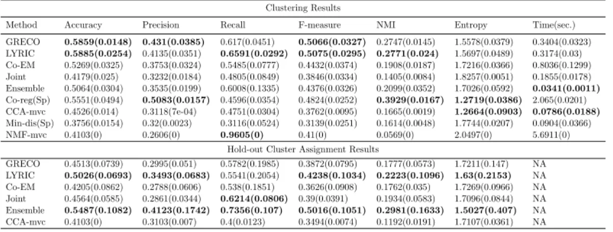
7.3.5 Empirical evaluation . . . 103
7.3.5.1 Baselines . . . 104
7.3.5.2 Datasets . . . 106
7.3.5.3 Results . . . 107
7.4 Conclusion . . . 115
Chapter 8. Conclusions and Future Work 117 8.1 Conclusions . . . 117
Appendices 121
Appendix A. Phenotyping using Grounded NMF 122
A.1 Phenotype sparsity . . . 122 A.2 Sample phenotypes for baseline models . . . 123 A.3 Augmented mortality prediction . . . 134
Appendix B. Explainability Using Manifold Constrained
Ex-amples 135
B.1 xGEMs for MNIST . . . 135 B.2 Case Study: Evaluating Model Training Progression . . . 137
Appendix C. Constraints based Clustering 138
C.1 Derivation of Variational Inference for Weighted Sum of Diver-gence Minimization . . . 138 C.2 Proof that aggregation in E-step can be solved in parallel over
samples . . . 139 C.3 M-step for Standard Mixture Models . . . 140 C.4 Formulae of Evaluation Metrics: . . . 141
List of Tables
4.1 Target comorbidities . . . 34
5.1 Additional notation used in this chapter . . . 37
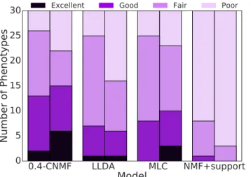
5.2 Relative Rankings Matrix: Each row of the table is the number of times the model along the row was rated strictly better than the model along the column by clinical experts, e.g., column 3 in row 2 implies that LLDA was rated better than MLC 12 times over all conditions by all experts. . . 43
5.3 30 day mortality prediction: 5–fold cross-validation performance of logistic regression classifiers. Classifiers for 0.4–CNMF and competing baselines (NMF+support, LLDA, MLC) were trained on the 30 dimensional phenotype loadings as features. Full EHR denotes the baseline classifier (`1-regularized logistic regression) using full ∼ 3500 dimensional EHR as features. CNMF+Full EHR denotes the performance of the `1-regularized classifier learned on Full EHR augmented with CNMF features (hyper-parameter was manually tuned to match performance of the Full EHR model). . . 46
5.4 Average F1-scores for Chronic Disease Prediction on MIMIC-II 51 5.5 Average F1-scores on low risk patients from MIMIC-II . . . . 51
5.6 Average F1-scores on high risk patients from MIMIC-II . . . . 51
6.1 Recalibrated Gender Classifier. . . 66
6.2 Confounding metric . . . 67
6.3 Confounding metric by gender . . . 67
7.1 LETOR Datasets Description . . . 91
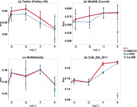
7.2 Twitter data (politics-uk, 3 views), best results obtained for γ = 0.01 for GRECO and LYRIC. Ensemble model, CCA-mvc, Min-dis(Sp) can cluster at most two views and marked NA oth-erwise. Co-reg(Sp), Min-dis(Sp) and NMF-mvc do not explic-itly compare hold-out cluster assignment results and have not been compared to for hold-out assignment performance. Top two methods w.r.t. each metric are highlighted. . . 111
7.3 Cornell (WebKB 2-views), best results obtained for γ = 0.1 for GRECO and γ →1 for LYRIC . . . 113 7.4 NUSWideObj Dataset (6 views), best results obtained for γ=
0.1 for GRECO and LYRIC. Since this data has three views that take negative values, we do not compare against NMF-mvc. CCA-mvc and Min-dis(Sp) cannot be extended for more than two views. . . 113 7.5 CUB-200-2011 (2 views), best results obtained for γ → 1 for
GRECO and LYRIC. Since this data has a view that takes negative values, we do not compare against NMF-mvc. . . 114
List of Figures
2.1 Latent Variable Model for Clustering . . . 18 5.1 Qualitative Ratings from Annotation: The two bars represent
the ratings provided by the two annotators. Each bar is a his-togram of the scores for the 30 comorbidities sorted by scores.
. . . 43 5.2 Phenotypes learned for ‘Psychoses’ (words are listed in order of
importance) . . . 44 5.3 Phenotypes learned for ‘Hypertension’ . . . 45 5.4 Top magnitude weights on (a) EHR and (b) CNMF features in
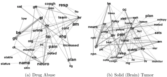
CNMF+Full EHR classifier . . . 48 5.5 Graph visualization of chronic conditions learned by theLabeled
APM model . . . 53 6.1 xGEMs versus Adversarial criticisms (Stock and Cisse, 2017),
for a parabolic manifold (shown in blue). Green points belong to class 1 and red points to class -1. The black trajectories in all figures are gradient steps taken by Algorithm 4 while the magenta trajectories correspond to adversarial trajectories de-termined by Equation 6.2 with p = ∞. Note that all decision boundaries in Figures (a) and (b) separate the data. The de-cision boundary is trained by optimizing a softmax regression using the cross-entropy loss function. . . 63 6.2 Example of bias detection. Target black-boxes:f1
φ and fφ2. g
∗
classifies points w.r.t. a. ˜x1 and ˜x2 are xGEMs corresponding
to x∗ for f1
φ and fφ2 resp. ˜x2’s attribute prediction (w.r.t g∗) is
the same as that ofx∗ while that of ˜x2 is different. Thus we say
that f1
φ is biased w.r.t. attribute a for sample x
6.3 We test whether ResNet models ˆf1
φ and ˆfφ2, both trained to
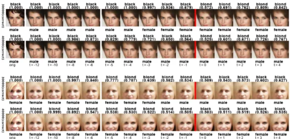
detect hair color but on different data distributions are con-founded with gender. Two samples for classifiers ˆfφ1 (first sub row) and ˆfφ2 (second sub row) are shown. The leftmost image is the original figure, followed by its reconstruction from the encoder Fψ. Reconstructions are plotted as Algorithm 4 (with
λ = 0.01) progresses toward crossing the decision boundary. The red bar indicates change in hair color label indicated at the top of each image along with the confidence of prediction. The label at the bottom indicates gender as predicted by ˆg. For both samples, classifier ˆf1
φ, trained on biased data changes the
gender (1st and 3rd rows) while crossing the decision boundary whereas the other black-box does not. . . 70 6.4 Confidence manifolds for a few data samples for black-box
mod-els 1 and 2. In each inset, this confidence manifold is traced dur-ing different stages of traindur-ing the black-box. In each inset, the legends denote: global training step (accuracy, parame-ter k, x0) denoting the global step at which the confidence
manifolds are plotted, and their corresponding logistic curve estimates and the overall black-box accuracy at that stage of training. Additionally, the curve shows whether the sample is misclassified at that training step. The top left and bottom left inset denote curves for a single sample – Sample 1 for the first and the second black-box respectively at different training stages. The true label for Sample 1 is ‘Black Hair’). The top right and bottom right curves show similar curves for black-box 1 and 2 respectively for Sample 2. The true label for Sample 2 is ‘Blond Hair’. . . 71 6.5 (a) and (b): 2d-Histograms of the parameters of the logistic
function fits to the confidence manifolds for a ∼4000 samples. 74 6.6 Reliability Diagram for Calibration stratified by (potentially
protected) attributes of interest (gender): A perfectly calibrated classifier should manifest an identity function. Deviation from the identity function suggests mis-calibration and can be used for model comparison when accuracy and other metrics are com-parable. . . 75 7.1 Visual representation of the proposed MR-CORE algorithm . 83
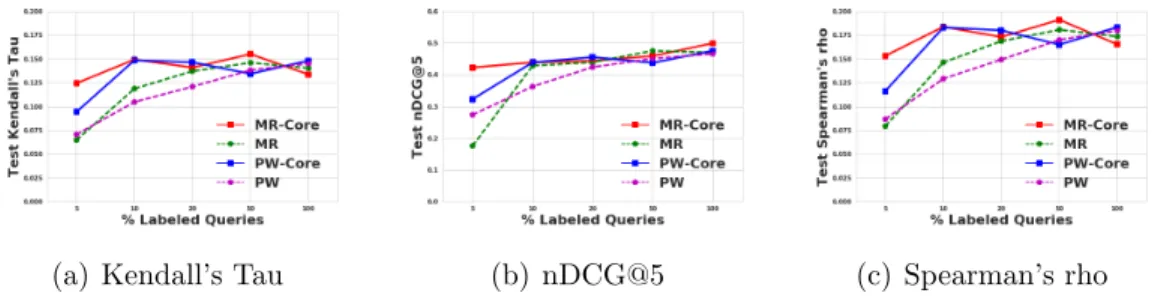
7.2 Ranking performance on held-out set of MR-Core when aug-mented using unlabeled data on MQ-2008. The x-axis sweeps over the percentage of queries used as labeled data from the training set. MR-Core: proposed model, PW-Core: point-wise model augmented with unlabeled data, MR: Supervised
MR, PW: Supervised pointwise model. . . 89
7.3 Ranking performance on held-out data when rank scores are only available as relevance/ pairwise scores on OHSUMED data. 89 7.4 Comparison to popular transductive ranking algorithms. The x-axis sweeps over the number of relevant documents in the la-beled set. TSVM: Transductive SVM,ssRankBoost: Trans-ductive Boosting for LeTOR. . . 90
7.5 Clustering Accuracy of GRECO and LYRIC w.r.t. logγ on (a) Twitter data (b) WebKB data (c) NUSWideObj data and (d) CUB 200 2011 data . . . 112
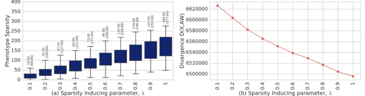
A.1 Sparsity–Accuracy Trade–off. Sparsity of the model is measured as the median of the number of non-zero entries in columns of the phenotype matrix A. (a) shows a box plots of the median sparsity across the 30 chronic conditions for varying λ values. The median and third–quartile values are explicitly noted on the plots. (b) divergence function value of the estimate from Algorithm 3 plotted against λ parameter. . . 123
A.2 Phenotype sparsity for baseline models . . . 124
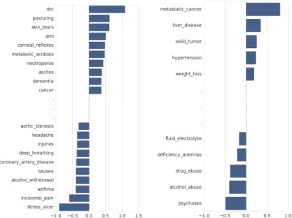
A.3 Learned Phenotypes for Liver Disease . . . 124
A.4 Learned Phenotypes for Solid Tumor . . . 124
A.5 Learned Phenotypes for Metastatic Cancer . . . 125
A.6 Learned Phenotypes for Chronic Pulmonary Disorder . . . 125
A.7 Learned Phenotypes for Alcohol Abuse . . . 125
A.8 Learned Phenotypes for Diabetes Uncomplicated. . . 126
A.9 Learned Phenotypes for Diabetes Complicated . . . 126
A.10 Learned Phenotypes for Peripheral Vascular Disorder . . . 126
A.11 Learned Phenotypes for Renal Failure . . . 127
A.12 Learned Phenotypes for Other Neurological Disorders . . . 127
A.13 Learned Phenotypes for Cardiac Arrhythmias . . . 127
A.14 Learned Phenotypes for Drug Abuse . . . 128
A.16 Learned Phenotypes for AIDS . . . 128
A.17 Learned Phenotypes for Fluid Electrolyte Disorders . . . 129
A.18 Learned Phenotypes for Rheumatoid Arthritis . . . 129
A.19 Learned Phenotypes for Lymphoma . . . 129
A.20 Learned Phenotypes for Coagulopathy . . . 130
A.21 Learned Phenotypes for Obesity . . . 130
A.22 Learned Phenotypes for Pulmonary Circulation Disorder . . . 130
A.23 Learned Phenotypes for Valvular Disease . . . 131
A.24 Learned Phenotypes for Peptic Ulcer . . . 131
A.25 Learned Phenotypes for Congestive Heart Failure . . . 131
A.26 Learned Phenotypes for Hypothyroidism . . . 132
A.27 Learned Phenotypes for Weight loss . . . 132
A.28 Learned Phenotypes for Deficiency Anemias . . . 132
A.29 Learned Phenotypes for Blood Loss Anemia . . . 133
A.30 Learned Phenotypes for Depression . . . 133
A.31 Weights learned by the CNMF+Full EHR classifier for all fea-tures. The weights shaded red correspond to phenotypes. . . . 134
B.1 xGEMs for MNIST data. Gθ : R100 → R28×28 is a VAE while the target black-box is a softmax classifier. Each row shows a manifold constrained exampletransition for a single digit (la-beled ‘orig’). The gray vertical bars indicate transition to the target label ytar. Reconstructions in each row are intermediate reconstructions obtained using Algorithm 4. The confidence of the clas prediction is shown in parentheses for each reconstruction.135 B.2 Training progression for celebA face image for the CNN+lrn model. . . 136 B.3 Training progression for celebA face image for the ResNet model.137
Chapter 1
Introduction
With wider applications of machine learning in e–commerce, web search, clinical healthcare, criminal justice platforms and systems, a few critical prac-tical challenges have come to the fore. These challenges remain a primary reason for a lack of trust as well as a hindrance to wider acceptance of machine learning based algorithms in practice. We discuss three of these challenges in the following and discuss how mechanisms formulated in this dissertation can be used to address them.
1.1
Interpretable machine learning
For application domains like clinical healthcare and criminal justice sys-tems, interpretability of machine learning algorithms is critical. Interpretabil-ity refers to designing learning and inference mechanisms to generate outcomes that are understandable to human or domain experts and are at acceptable levels of abstractions.
1.2
Explainable machine learning
Certain state of the art machine learning models, like deep learning methods, involve learning millions of parameters. Understanding such com-plex models requires a sophisticated understanding of model behavior and is
therefore inaccessible to a consumer of the model. Such models have become black-box models. It is therefore necessary to develop equally sophisticated mechanisms that probe such models to understand and summarize their be-havior using abstractions that are accessible to non–experts.
1.3
Semisupervised machine learning
Typically, supervised learning algorithms learn a functional mapping from attributes over samples to a known target score or categorical label. Col-lecting the target score/labels is called annotation. This requires expensive human as well as engineering resources for large datasets. Semisupervised learning refers to learning reliably in the absence of reliable and/or limited expert annotation. For instance, it is desirable to rank patients at a caregiv-ing facility in order of their risk of outcome like mortality. It is increascaregiv-ingly difficult to get such subjective scores as it requires expensive clinical exper-tise. However, heterogeneous sources of information are sometimes available to describe a single data point. For instance, patients in a hospital can be described by their prescription information, claim information, as well as lab test information.
1.4
A Constraint Based Framework
This dissertation focuses on developing a common framework to build interpretable, explainable models as well as to learn reliably when little to no annotation is available. We rely on a framework that assumes such observa-tions can be represented in an unobserved low–dimensional space. This space is called the latent space and the corresponding class of models are known
as latent variable models. Characterizing such a latent space, the distribu-tions over the latent space, as well as the realizadistribu-tions corresponding to the observed samples are the main tasks of an associated learning algorithm. We demonstrate that constraining different aspects of the latent space allows one to (i) encourage models to satisfy specific interpretability criterion (ii) probe complex black-box models to summarize model behavior, and (iii) leverage heterogeneous data sources in lieu of expert annotation to learn reliably at scale.
The first part of the dissertation demonstrates a framework that con-strains realizations of latent variables. The corresponding learning algorithms are augmented to impose these constraints during training. Tractable ap-proximations are used when exact imposition of constraints is infeasible. We demonstrate the utility of our mechanism on our working application – au-tomated phenotyping of chronic conditions from Electronic Health Records (EHRs). We rely on two existing latent variable frameworks, namely, prob-abilistic graphical models (Wainwright and Jordan, 2008) and non–negative matrix factorization (Lee and Seung, 1999) to demonstrate our constraining formulation. Next, we demonstrate how a constrained generative model can be used to probe complex supervised black-box models to generate explanations or summaries of model behavior. Finally, we demonstrate how distributions over latent variables can be constrained as a means to leverage heterogeneity of data sources. This mechanism allows us to leverage multi–modal data sources to learn without expensive supervision. This is applied usingco–regularization for clustering as well as for learning to rank (LeTOR) (Trotman, 2005) algo-rithms.
mathematical constructs used to propose the constraining mechanisms. In particular, the latent variable models used to demonstrate the explainabil-ity mechanisms are variational auto–encoders (VAEs) (Kingma and Welling,
2013), probabilistic graphical models (Koller and Friedman, 2009), and latent factor models, specifically non–negative matrix factorization (NMF) (Lee and
Seung, 2001). These modeling paradigms are introduced in detail. We
intro-duce a latent variable paradigm for clustering, called mixture models. Finally, a learning to rank (LeTOR) framework based on Generalized Linear Mod-els (McCullagh, 1984) is introduced. All models and associated training and inference mechanisms are substantially generalized in the following chapters to incorporate appropriate constraints.
Chapter3details the paradigm of learning interpretable latent variable models using constraints. To do so, we first review existing literature toward developing interpretable and explainable machine learning. We contextualize the proposed formulation’s relevance to existing literature on interpretability and explainability models. The chapter focuses on introducing conditions that could be imposed on a machine learning model to encourage it to be inherently interpertable given the application domain and an abstraction level. Next, the general mechanism of constraining individual realizations of latent variables is described for latent space models (to specifically encourage interpretability), including augmenting the learning and inference mechanisms. Finally, we pro-pose an instance of such constraints (calledgrounding) that are relevant to our application for phenotyping chronic conditions using EHR data. We discuss some inherent trade-offs of these constraints in terms of model performance and/or interpretability.
phe-notypes for chronic conditions of an ICU population using Electronic Health Records. This is our working example to demonstrate the utility of our con-straining formulation for enhancing interpretability of ML models. We review existing phenotyping algorithms, and discuss how the proposed formulation addresses existing issues of identifiability and interpretability for phenotyping. We further discuss how EHRs, specifically clinical notes are pre–processed to generate observations as well as weak diagnoses required to imposegrounding constraints discussed in Chapter3.
Chapter 5 demonstrates how the grounding framework is applied to – (i) a NMF framework, and (ii) admixture of PMRFs (Inouye et al.,2014a) . A new algorithm for learning as well as inference is proposed in each case drawing onMaximum-a-Posteriori estimator, and an Alternating-Minimization frame-work (Koren et al., 2009). The proposed models are evaluated qualitatively and quantitatively. Qualitatively, domain experts (clinicians) were asked to evaluate the quality of the learned phenotype representations based on their relevance of the target conditions as well as their discriminative ability relative to well known baselines. Finally, the phenotype representations are evaluated for their predictive power in determining patient outcomes (30-day mortality outcomes) as a quantitative evaluation of their utility on a down-stream eval-uation. We conclude this chapter by discussing some limitations of learning phenotypes without accounting for interventional information.
Chapter6proposes xGEMs ormanifold constrained exemplars, a frame-work to understand black–box classifier behavior by exploring the landscape of the underlying data manifold as data points cross decision boundaries. To do so, we train an unsupervised generative model – treated as a proxy to the data manifold. We summarize black-box model behavior quantitatively by
generating perturbations of existing samples constrained along the data mani-fold. Constraining these perturbations requires restricting the latent variables by transforming them using the generative function mapping. We demon-strate xGEMs’ ability to detect and quantify observed attribute confounding in model learning and also for understanding the changes in model behavior as training progresses.
Chapter 7 is devoted to leveraging heterogeneous data sources using constraints, in order to effectively learn in the absence of annotation. We do so by effectively constraining distributions over latent spaces and/or latent variables themselves. The first part of the chapter develops a latent variable framework specifically for clustering. In particular, we demonstrate that an effective choice of divergence function to constrain the distributions over the latent variables across heterogeneous data sources can help to learn a parti-tioning even when the individual data sources may be slightly biased w.r.t. the true clustering distribution. Two algorithms are proposed utilizing this choice of divergence based on variational inference (Wainwright and Jordan, 2008) for estimation. The proposed algorithms have been extensively evaluated on clustering document and social network data. The latter half of Chapter7 pro-poses to use heterogeneous sources to learn reliable ranking models when rank ordering is only available for a very few queries. This requires us to substan-tially generalize an existing listwise ranking framework known as Monotone Retargeting (Acharyya et al., 2012; Acharyya and Ghosh, 2014). We develop novel constraints to enforce agreement across rank–orderings generated by het-erogeneous data sources, specifically those of unlabeled queries. Consequently, this ranking framework is evaluated on semi–supervised LeTOR tasks for in-formation retrieval applications.
We conclude in Chapter 8 with some directions for future work fo-cusing on incorporating structural and domain constraints that inform causal influences for generating interpretable and explainable models.
Chapter 2
Background
We first introduce necessary notation that will be used throughout this dissertation.
2.1
Notation
A vector of dimension d is denoted byx∈Rd. A matrix of dimensions
d×k is denoted by a bold caps letter, e.g. X ∈ Rd×k. The space of non-negative reals is denoted byRd+×k. xj is thejth column of matrixX while x(i) denotes the ith row of matrix X. x
ij is the entry in the ith row and the jth column of X.
The set of indices {1,2,· · · , m} is denoted by [m]. ∆d−1 is the Simplex
in dimension d, ∆d−1 ={x∈Rd
+ :
P
xi = 1}. Similarly, a λ–∆d−1 (called the lambda-Simplex) in dimension d is the set λ–∆d−1 ={x∈
Rd+ :
P
xi =λ}. supp(x) is the support of vectorx. That is, supp(x) ={i:xi 6= 0}. A generic set is denoted by sans–serif letter C. The set of all vectors isotonic to a vector y is denoted by R↓y, i.e. it denotes the set of all vectors that result in the same rank order as y.
We focus on the class of latent variable and latent factor models in order to demonstrate the utility of our constrained based algorithms for inter-pretability, explainability, and semi–supervised learning. The following builds
the necessary background to formulate our models.
2.2
Non-Negative Matrix Factorization
Non–negative matrix factorization (NMF) is a latent factor model. NMF approximates observational data (represented in non–negative matrix form) as a factorization of two low–rank non–negative matrices. The quality of the approximation is measured using a divergence function defined below. 2.2.1 Bregman divergences
Bregman Divergences is a class of divergence functions closely related to the exponential family distributions, that is, there is a one–to–one map-ping between regular exponential family distributions and the class of regular Bregman Divergences (Banerjee et al., 2005b).
Definition 2.2.1. Let f : dom(f) → R be a continuously differentiable strictly convex function defined on the closed convex setdom(f). TheBregman Divergence between x, y ∈dom(f) is defined as:
Bf(x, y) =f(x)−f(y)− h∇f(y), x−yi (2.1) For two matricesX,Y∈RN+×d, the divergence D(X,Y) is given by:
D(X,Y) = X ij
B(xij, yij) (2.2) We restrict the class of divergence functions to belong to Bregman di-vergences (Definition 2.2.1) for formulating non–negative matrix factorization for interpretability given their attractive properties like convexity and associ-ations with the exponential family distributions.
2.2.2 Non–negative matrix factorization
Let X ∈ RN+×d be a matrix with non–negative entries. Non–negative matrix factorization approximates the observation matrix as a factorization of two low–rank non–negative matrices. Let A ∈RN+×K and W∈ Rd+×K be two rankK matrices. Then generalized non–negative matrix factorization aims to find estimates ˜A and ˜W via constrained minimization of the following cost function:
˜
A,W˜ = arg min
A∈RN+×K,W∈Rd+×K
D(X,AWT) (2.3)
whereCAand CW denote appropriate constraints on the non–negative factors, either obtained via supervision or appropriate domain constraints. The choice of the divergence function D(X,Y) is determined by the type of data comprising the observation matrixX and the probabilistic assumptions made for data generation. The choice ofK is determined by empirical evaluation on a validation set or can be determined from the application domain.
2.2.3 Alternating–Minimization algorithm
In order to estimate the low–rank factor matricesA and W, an effec-tive and scaleable algorithm is called Alternating Minimization (Koren et al.,
2009). Without any constraints on the estimates of A and W other than non–negativity, Algorithm 1can be used to obtain the estimates.
2.3
Admixtures of Markov Random Fields
We demonstrate the utility of our domain specific interpretable models by applying it to a probabilistic latent variable model. In particular, we restrict to the class of admixture of Markov Random Fields, detailed in the following.
Algorithm 1 Alt-Min for NMF Input: X. Initialization: A(0)
while Not converged do
W(t) ←arg minW∈R+d×KD(X,A(t−1)W)
A(t) ←arg minA∈R+N×KD(X,AW(t))
end while
2.3.1 Admixture models
Admixture models were primarily introduced to model heterogeneity in genetic linkage analysis data. The probabilistic assumptions underlying ad-mixture models is as follows. LetKbe the number of populations (or generally mixture components). Let 0≤wk ≤1 be the proportion with which mixture
kcontributes to the observed population and let Θk parametrize the probabil-ity of observing a sample from the kth component of the mixture (denoted by
p(x; Θk)). Letx∈Rd+ be the random variable representing observation. Then
an admixture model is represented by the following generative process: xm ∼p(x;X
k
wmkΘk)∀m∈[N] (2.4)
where N is the total number of samples in the observation. 2.3.2 Poisson Markov Random Fields (PMRFs)
Poisson Markov Random Fields (PMRFs) (Yang et al.,2013), are markov random fields defined in order to incorporate correlation between multivari-ate Poisson random variables. Let x ∈ RV be a V dimensional count vector drawn from a PMRF. The distribution of x can be parametrized by θ ∈ RV
and Θ∈RV×V and is given by1: p(x|θ,Θ)∝exp{θTx+xTΘx− V X v=1 ln(xv!)} (2.5) As can be seen from Equation (2.5), a PMRF explicitly accounts for potential correlation between the xv vectors. Θ plays a similar role as the precision matrix as in a multivariate Gaussian distribution i.e. encoding con-ditional independence structure. Note that (Inouye et al.,2014a) use a slightly modified distribution to account for positive correlations based on (Yang et al.,
2013). An important distinction here is that in comparison to the multinomial distribution, used in LDA (Blei et al.,2003), PMRFs allow to model positive as well as negative correlations between words in the vocabulary. A multinomial distribution accounts for weak negative correlations by fixing the total count of trials and does not model correlations explicitly (Inouye et al., 2014a). 2.3.3 Admixtures of PMRFs (APM)
APM may be considered to be an undirected graphical model based analogue of LDA. Both model a document as a bag-of-words. Each document is represented as a vector, so each dimension counts the number of times a given word appears in the document. APMs are based on Poisson Markov Random Fields (PMRFs) (Inouye et al., 2014a), to incorporate correlation between multivariate Poisson random variables.
Consider K PMRFs - one for each topic, with parameters {θk,Θk}. Topic models assume that a document is composed of words from multiple
1Note that proportionality signs imply appropriate normalization so that the distribution
topics. Therefore, to generate each document n in a corpus of N documents, each consisting of one or more of K topics, one can follow the following gen-erative procedure using PMRFs:
For eachn ∈N,
• Sample wn ∈ ∆K according to a Dirichlet distribution p(w|α), where
α ∈RK, α >0 and ∆Kindicates theK−1 dimensional simplex (see2.1). These are known as the admixing weights.
• Let θn =PKk=1wnkθk and Θn=PKk=1wnkΘk. Since the ‘weight’ vector
wn lies on the simplex, θn and Θn are convex combinations of the topic parameters.
• The document xn is generated by sampling from a new PMRF with parameters {θn,Θn}.
The complete distribution of the corpusXconsisting of independent document samplesxn, each drawn from a PMRF, is given by,
p(X|θk,Θk)∝ N Y n=1 p(xn|θn= K X k=1 wnkθk,Θn= K X k=1 wnkΘk) (2.6)
where each entity in the product on the right hand side can be modeled ac-cording to Equation (1). In addition, prior probabilities p(θk,Θk|β) may be imposed on the parameters θk and Θk, ∀k ∈ {1,2, ..., K} (Inouye et al.,
2014a). β can thus be considered as a tuneable hyperparameter.
2.3.4 Maximum-a-Posteriori algorithm for PMRFs
Inouye et al.(2014a) propose to obtain aMaximum-a-Posteriori (MAP)
scaleable approach for the MAP estimation procedure is proposed in Inouye
et al.(2014b). We build upon this procedure for incorporating topic–level
su-pervision. The unsupervised MAP estimation procedure involves alternating co–ordinate descent type optimization. One equation updates parameters of the topics i.e. the PMRF parameters with constant admixing weights and the other equations updates the admixing weights with constant topic parameters. Letzi = [1, xTi ]T,φkv = [θkv, Θkv] wherev indexes thevthrow ofθkand Θk∀k ∈ {1,2, ..., K}. In addition letΦv = [φ1v, φ2v, ...φKv]. The optimization problem is given by the following two equations optimized in an alternating manner. arg min Φv − 1 n V X v=1 [tr(ΨvΦv)− N X i=1 exp (zTi Φvwi)]+ λ V X v=1 kvec(Φv)−ik1 (2.7) arg min w1,...wn∈∆K − 1 n N X i=1 [ΨiTwi− V X v=1 expzTi Φvwi] (2.8) where Ψv and Ψv can be calculated from observations X. The subscript −i indexes theithsubvector of the vectorized form of Φ
v. The above equations are iteratively minimized to obtain a local optimum over the PMRF parameters Φv and the admixing weights w1, ..., wn. Equation (2.7) updates the PMRF parameters when the admixing weights are fixed and the admixing weights are updated in Equation (2.8) with PMRF parameters fixed from latest estimates of (2.7).
2.4
Deep Generative Models
Generative Models can be described as stochastic procedures that gen-erate samples (denoted by the random variable x∈Xd) from the data distri-butionp(x) without explicitly parameterizing p(x). The two most significant types are the Variational Auto–Encoders (VAEs) (Kingma and Welling,2013) and Generative Adversarial Networks (GANs) (Goodfellow et al.,2014a). Im-plicit generative models generally assume an underlying latent dimension z∈ Rk that is mapped to the ambient data domain x∈Rd using a deterministic functionGθ parametrized byθ, usually as a deep neural network. The primary difference between GANs and VAEs is the training mechanism employed to learn function Gθ. GANs employ an adversarial framework by employing a discriminator that tries to classify generated samples from the deterministic function versus original samples and VAEs maximize an approximation to the data likelihood. The approximation thus obtained has an encoder-decoder structure of conventional autoencoders. We use VAEs for our explainabil-ity experiments. One can obtain a latent representation of any data sample within the latent embedding using the trained encoder network. While GANs do not train an associated encoder, recent advances in adversarially learned inference like BiGANs (Dumoulin et al., 2016; Donahue et al., 2016) can be utilized to obtain the latent embedding. In this work, we assume access to an implicit generative model that allows us to obtain the latent embedding of a data point.
2.5
Learning to Rank (LeTOR)
Learning to Rank or LeTOR models consider the problem of estimating a preference order over a set of items (Liu,2009). For instance, ranking a fixed
set of web documents in order of relevance to a search query. Listwise ranking requires to rank order a list of objects in order of preference or relevance. We briefly discuss the listwise LeTOR algorithm used in this work below.
2.5.1 LeTOR using Monotone Retargeting (MR)
MR is a supervised listwise ranking technique that learns a General-ized Linear Model (GLM) on scores/ranks over a set of objects. MR leverages the idea that only the ordering induced by the scores over items are of con-sequence in a LeTOR framework. MR thus searches for parameter estimates over all monotonic transformations of the scores. That is, Acharyya et al.
(2012) observe that listwise ranking only aims to learn an appropriate permu-tation over items in a query which can be interpreted as learning a scoring function on any monotonic transformation of the original scores to preserve order over items. This allows for parameter estimation of the GLM based cost function by fitting over target score vectors in addition to all scores isotonic to the original – called retargeting. Allowing such a retargeting has signifi-cant advantages under model–misspecification by providing more flexibility to under–specified models. For instance, linear GLMs can be used to fit integer scores (most commonly used in practice for annotating) by searching for an appropriatelyretargeted set of scores. Further, MR exploits the fact that the set of all vectorsisotonic with the scores associated with a group of items in a query is a convex cone. Thus, the listwise ranking can be formulated as a biconvex optimization problem that alternately estimates the scoring function parameter and retargets the scores within the appropriate convex cone.
Specifically (notation is consistent with that of Acharyya et al.(2012)), letQ={q1, q2,· · · , qt}be a set of queries each consisting of items Vqi ⊂V, i∈
Algorithm 2 Monotone Retargeting (MR) Input: Xq ∈R|Vq|×d,yq, q ∈Q;φ
Initialize w,rq, q ∈Q: while Not converged do
Solve using parameter estimation for GLMs: w= arg minw∈Rd P q∈QDφ(rqk∇φ−1(Xqw)) Retargeting step: rq = arg minrq∈R↓yq Dφ(rqk∇φ −1(X qw))∀q∈Q in parallel end while
[t] to be ranked. Let Xq ∈ R|Vq|×d, q ∈ Q be the feature matrix associated with these items and let yq be scores representing the ranking permutation. Let Dφ(x,y) be an appropriate2 distance like function between two vectors x,y ∈ Rd. Finally let R
↓yq represent the convex cone of all vectors that are
isotonic to yq, i.e. all vectors that result in the same rank order asyq. Then MR for listwise ranking can be formulated to estimate a function parametrized by w ∈ Rd that fits any monotonic transformation of the score vector. That is, ˜ w= arg min w∈Rd,r q∈R↓yq,q∈Q X q∈Q Dφ(rq,∇φ−1(Xqw)) (2.9) MR uses Bregman Divergences (see Definition 2.2.1) in order to mea-sure the quality of the fit to the rank scores. The estimation algorithm is an alternating minimization procedure comprising of a standard parameter esti-mation step as that of Generalized Linear Models (GLMs) and a ‘Retargeting Step’ solved using the Pool-Adjacent Violators (PAV) algorithm (Best and
Chakravarti,1990). The retargeting step allows to fit the GLM over any
vec-tor isotonic to the target scores and hence have to be recomputed every time
πn zn xn
N
Ψ
Figure 2.1: Latent Variable Model for Clustering
the GLM parameter estimate updates. The complete algorithm for LeTOR using MR is summarized in Algorithm 2. The formulation easily allows to account for partial ordering by augmenting the algorithm with a simple per-mutation step (Acharyya et al.,2012).
Extensions of MR, called Margin Equipped MR (MEMR) mitigate is-sues like degeneracy of solutions by allowing to add margins within the ranking scores and augmenting the cost function using`2–regularization to ensure joint
convexity.
2.6
Clustering
Clustering is the task of estimating a partition of the data given finite samples from the data distribution. Without further assumptions, this prob-lem is ill–posed. We formulate our clustering probprob-lem using a probabilistic latent variable framework. Figure2.1show the corresponding graphical model that induces appropriate probabilistic dependencies to describe the generative process of the clustering formulation. Specifically,zis the latent (unobserved) random variable representing cluster membership for any sample. πn is the prior probability of a sample n belonging to one of K clusters. xn is the ob-served sample that is generated as follows: 1.zn ∼p(z;πn) 2. xn ∼p(x; Ψzn)
A categorical distribution is a discrete distribution over outcomes ω ∈ [K] parameterized by θ ∈ ∆K so that P r(ω = k) = θk. It is a member of the exponential family of distributions. The natural parameters of categorical distribution are logθ = (logθk)k∈[K] and sufficient statistics are given by the
vector of indicator functions for each outcome ω ∈ [K], denoted by z(ω) ∈ {0,1}K with:
zk(ω) = (
1, if ω =k,
0, otherwise.
In the proposed generative model,zis modeled as a categorical variable. Given two categorical distributions p(ω) and q(ω), describing the dis-tribution over the categorical random variable ω, the divergence of p(ω) from
q(ω), denotedD(p(ω)kq(ω)), is a non-symmetric measure of the difference be-tween the two probability distributions. TheKullback-Leibleror KL-divergence is a specific divergence denoted by KL(p(ω)kq(ω)) and is defined as follows.
KL-divergence of p(ω) from q(ω) is given by:
KL(p(ω)kq(ω)) = Ep(ω)[ logp(ω)−logq(ω) ] (2.10)
This is also known as the relative entropy betweenp(ω) andq(ω). The relative entropy is non-negative and jointly convex with respect to both arguments. Further, we have that KL(p(ω)kq(ω)) = 0 iff p(ω) =q(ω), for allω. Note that the KL–divergence is a special case of the Bregman Divergence2.2.1.
The R´enyi divergences (R´enyi, 1960) are a parametric family of diver-gences with many similar properties to the KL-divergence. Since our focus is on using these divergences to measure distances of distributions over clus-ter labels, we will focus on R´enyi divergences for distributions over discrete random variables.
Definition 2.6.1. (van Erven and Harremo¨es, 2012) Let p, q be two dis-tributions for a random variable ω ∈ [K]. The R´enyi divergence of order
γ ∈(0,1)∪(1,∞) of p(ω) from q(ω) is, Dγ(p(ω)kq(ω)) = 1 γ−1log XK ω=1 p(ω)γq(ω)(1−γ) (2.11)
The definition may been extended for divergences of other orders like
γ = 0, γ → 1, and γ → ∞ (van Erven and Harremo¨es, 2012). R´enyi
di-vergences are non-negative ∀γ ∈ [0,∞]. In addition, they are jointly convex in (p, q) ∀γ ∈ [0,1] and convex in the second argument q ∀γ ∈ [0,∞]. As discussed in the comprehensive survey of R´enyi divergences byvan Erven and
Harremo¨es(2012), many special cases of other commonly used divergences are
recovered for specific choices of γ. For example, γ = 12 and γ = 2 give R´enyi divergences which are closely related to the Hellinger and χ2 divergences, re-spectively, and the KL-divergence is recovered as a limiting case when γ→1. For the rest of the manuscript, we will abuse notation slightly and usep(ω) and
p(z) interchangeably to denote the same categorical distribution over outcomes in [K].
2.7
Discussion
The following chapters unify all models under the latent variable frame-work and discusses how different aspects of these models can be constrained for improved interpretability, explainability and semisupervised learning.
Chapter 3
Interpretable Latent Variable Models
Interpretability and Explainability of machine learning models are be-coming increasingly imperative as they become widely applied to domains like the criminal justice system (Angwin et al., 2016), clinical healthcare (
Calla-han and Shah,2017), etc. The COMPAS (Angwin et al., 2016) system learns
recidivism scores to determine pre–trial bail and detention. Clinical interven-tions determined using machine learning algorithms can affect patient lives, thus making it important for caregivers to provide explanations for such in-terventions. Such applications that substantially impact human lives have motivated regulatory agencies like the EU Parliament1 to codify a right to data protection and “obtain an explanation of the decision reached using such automated systems2”.
Challenges in this domain are compounded by a lack of characterization of what constitutes a sufficient explanation (Lipton,2016). Additionally, differ-ent levels of abstractions are necessary depending on the stakeholders (Miller,
2017). For instance, explanations of interesting behaviors that may assist a data science practitioner are vastly different from those that help caregivers and/or patients make better interventional choices.Doshi-Velez(2017);Miller
(2017) have recently attempted to characterize such abstractions from the
1in collaboration with the EU Commission and the Council of the Eurpean Union
perspective of the desired outcome as well as drawing from extensive social scientific literature on how humans process explanations. Generally, there is ground to believe that such a suite of methods can be useful not only help im-prove understanding of opaque models3 (Higgins et al., 2016;Karpathy et al., 2015) but can also uncover biases (inherent in the data) that models pick up on e.g. learned gender and racial biases (Bolukbasi et al., 2016).
3.1
Related Work
While generally referred to interchangeably, we distinguish interpretable machine learning models as those that learn easily understandable outcomes to a target user. On the other hand, explainability tools refer to models that can be used to provide post–hoc explanations of pre–trained complex models. Some models have been exclusively developed in order to serve as diagnostic toolsto ‘explain’ existing or pre–trained models. Notable ones are described in the following. We describe existing work relevant to developing interpretable models, as well as explainable models in the following. The rest of the chapter is thereafter devoted to exposing the utility of interpretable machine learning using constraints in latent variable models. The explainability exposition is relegated to Chapter 6.
3.1.1 Interpretable machine learning
Interpretable ML methods focus on developing machine learning mod-els whose outcomes inherently satisfy a specific interpretability criterion. Usu-ally, such criterion tend to be domain as well as application specific. Notable
among these are methods that use tools based on model distillation (Hinton
et al., 2015) and attention based mechanisms (Ba et al., 2014). As a
work-ing example, we focus on interpretable models that have been developed for clinical healthcare. The main goal of interpretability of ML models in clinical decision making is to expect the model to learn clinically relevant, physiolog-ically plausible, and represented in a form or abstraction that is understand-able to clinical experts. For instance, Choi et al. (2016) use attention based mechanism for time series data for training explainable models for outcome prediction, whileChe et al.(2016) use model compression and distillation, sim-ilarly for outcome prediction for an ICU patient population. This dissertation focuses on phenotyping (Pathak et al., 2013) of co-occurring chronic condi-tions for ICU patients as the working application for developing inherently interpretable models. EHR driven phenotypes are concise representations of observable clinical traits that can facilitate reliable querying of individuals from the EHRs (NIH Health Care Systems Research Collaboratory, 2014). While most interpretability mechanisms described above focus on supervised models, EHR driven phenotype has to be posed as an unsupervised learning problem with availability of weak or noisy supervision.
3.1.2 Explainable machine learning
Stock and Cisse (2017); Kim et al.(2016); Gupta et al.(2016);
Lund-berg and Lee (2017) develop models specifically to explain classifier decision
and behavior. Different methodologies are used in order to provide such post-hoc explanations. For instance Elenberg et al. (2017); Kim et al. (2016) se-lect prototypes/examples and/or groups or semantically relevant features from the training dataset as a means to detect failure cases of supervised models.
It may happen that points that explain a model according to the predeter-mined criterion may not exist in the dataset. In order to solve this problem we propose a method to generate samples by approximating the data man-ifold using a generative model like a GAN (Goodfellow et al., 2014a) or a VAE (Kingma and Welling,2013).Stock and Cisse (2017) use the adversarial attack paradigm (Goodfellow et al.,2014b) to generate prototypes and/or ex-amples where the classifier shows interesting failure cases (called criticisms). Another class of methods locally approximate complex classifiers with a sim-pler model class (e.g. linear) in order to generate explanations (Lundberg and Lee,2016;Ribeiro et al.,2016;Shrikumar et al.,2016;Bach et al.,2015). These methods inherently assume a trade–off between model complexity and explain-ability. Empirically, it is observed that simpler model classes also tend to be empirically sub–par. Thus such models inherently assume a trade-off between model performance and explainability.Li et al. (2015); Selvaraju et al.(2016) focus on understanding the workings of different layers of a deep network and studying saliency maps for feature attribution (Simonyan et al.,2013;Smilkov et al.,2017;Sundararajan et al.,2017). Saliency methods, while powerful, can be demonstrated to be unreliable without stronger conditions over the saliency model (Kindermans et al., 2017;Adebayo et al.,2018).Koh and Liang (2017) use influence functions, motivated by robust statistics (Cook and Weisberg,
1980) to determine importance of each training sample for model predictions.
3.2
Latent Variable Models for Interpretability
This dissertation focuses on the class of latent variable models to pro-pose the interpretability and explainability framework. We posit that con-straining latent variable models appropriately can allow to learn models that
generate interpretable outcomes and to explain existing ML models in a post–hoc manner. Probabilistic graphical models, latent factor models like matrix fac-torization, and implicit generative models are a few well known examples within this class. In particular, this framework offers the following advan-tages in terms of its amenability to formulating explainable and interpertable machine learning models:
• Latent variable models induce an associated probabilistic generative pro-cedure for the observed data. Constraining the generative process allows to easily encode constraints that make the model (say physiologically) plausible and therefore more interpretable.
• In particular, constraints on the model class, parameters of the model class, as well as the generative procedure itself can be imposed for indi-vidual observational samples, lending the model to be more amenable to generating individualized/personalized explanations whenever necessary. • Scaleable learning and inference procedures can be non–trivially ex-tended for this class of models that can be augmented seamlessly to incorporate any relevant constraints.
• Specifically for the working example of phenotyping chronic conditions, this framework allows to learn phenotypes for all chronic conditions si-multaneously (a modeling requirement since such chronic conditions tend to co-occur or are comorbidities (Elixhauser et al., 1998)).
The following describes a general framework to formulate interpretable latent variable models by constraining latent variable models. A detailed mo-tivation for constrained based models to (post-hoc) explain black-box models is deferred to Chapter 6.
3.3
Constraint Based Framework for Interpretability
Let x ∈ Rd be the random variable representing observations. Let z ∈ Rk, k << d represent the set latent (unobserved) variables that can well approximate the observationxvia functionfθ. That is, letfθ :Rk →Rddefine an approximation to the observations as a function of unobserved variablesz. Let L : Rd×d →
R+ determine the quality of such an approximation. A few
examples making this framework concrete in different settings are given below:
(a) Directed Graphical Model (b) Undirected Graphical Model
1. Probabilistic Graphical Models: A probabilistic graphical model is a framework to encode dependencies between a set of random variables and an associated realizable probabilistic distribution. Figure3.1(a)shows a graph-ical model that demonstrates the dependency between the latent variables z and the observational data x, while Figure 3.1(b)shows an undirected graph-ical model analogue encoding the dependency structure between latents zand observed variables x.
2. Latent Factor Models: Latent factor models is a class of models that expresses observations a linear combination of shared ‘factors’ or vari-ables, where both, the shared factors as well as the strength of the linear combinations are unknown (latent). We restrict to the class of non–negative matrix factorization in this study. Refer to background in Sec 2.2 for details.
In particular, the probabilistic assumptions induced in NMF can be repre-sented as the following. Let w ∈ Rk
+ be the latent variable representing the
unknown linear combinations or loadings while let the columns of the matrix A ∈ Rd×K
+ (denoted by a(k)) represent the common or shared factors across
observed samples. Then,
E[x|w] =Pk∈[K] a(k)wk (3.1) 3. Implicit Generative Models: Implicit Generative Models are generative models that map latent variable z to observed data x via a deter-ministic functionGθ without parametrizing the underlying stochastic process. Examples of such a deterministic function can be a deep neural network. Such models are usually trained either via a maximum likelihood procedure or an adversarial training procedure (see Sec 2.4) for more details.
To formulate interpretable models, we propose to impose model con-straints on 1. latent variables 2. model parameters 3. generative procedure or a combination thereof. We represent constraints on the latent variables as
Cz. Constraints on model parameters are represented as Cθ and that on the generative process can be described as part of model assumptions. In general, the optimization process can be formulated as the following:
˜ z,θ˜= arg min z,θ E [L(x, fθ(z))] s. t. z∈Cz,θ∈Cθ (3.2) 3.3.1 Augmented training
Without interpretability requirements, the loss function determining the quality of the approximation can be optimized with respect to model
pa-rameters without additional constraints. Specifically, in the absence of con-straints on latent variables, out-of-the-box training algorithms can be utilized for learning model parameters, which are of primary interest in general. How-ever, interpretability constraints on latent variables can be imposed by al-gorithms that allow to interleave model parameter estimation with imposing required constraints. Thus, we suggest that the class of algorithms that rely on model parameter estimation without marginalizing latent variables are more amenable to developing interpretable models via constraints. Typically such a class of algorithms follow the prescription of majorization–maximization (Hunter
and Lange, 2000) construct of algorithms and leverage the latent variable
in-ference framework to achieve tractability of an otherwise complex optimiza-tion algorithm. Examples of algorithms used in this dissertaoptimiza-tion for imposing interpretability constraints are 1. Expectation-Maximization 2. Variational In-ference (Wainwright and Jordan,2008) for the class of probabilistic graphical models, 1. Alternating–Minimization for latent factor analysis.
3.3.2 Grounding mechanism
One way to impose constraints, that is specifically useful for the phe-notyping application is described in the following. The mechanism, called grounding, is extensively evaluated for different models in the following chap-ters. The mechanism involves enforcing constraints on the latent variables and/or on the model parameters.
1. Support Constraints: This set of constraints is imposed on the sup-port of individual samples of the latent variablez. Letj ∈[N] index individual sample observations. We assume a setCj can be determined from side informa-tion such that aninterpretable model would only allow for estimates satisfying:
supp(z(j)) =C
j. We motivate this using the non-negative matrix factorization setting in the context of phenotyping. The non-negative rank–K factorization of X is said to be ‘grounded’ to K target comorbidities by constraining the support of loadings w(j) corresponding to patient j using weak diagnosis C
j that can be easily computed from administrative patient data. This amounts to restricting the set of allowable linear combinations that can describe an observed phenotype for any patient sample. As we shall see in Chapter 5, if
Cj are accurate, then this constraint follows from the definition of phenotypes. 2. Sparsity Constraints: In many applications, model parameter esti-mates are eventually consumed by domain experts for final decision making. Thus, it is desirable that the phenotype representations be easily interpretable for human experts. Sparsity of the model parameter θ is used as a mea-sure of domain specific interpretability. For the case of phenotyping using non–negative matrix factorization, sparsity is induced using the scaled sim-plex constraints on the columns of A. Associated with the constraint is a tuneable parameter λ >0 to encourage sparsity of phenotypes.
3.4
Discussion
Advantages of such constraints are 1. they follow easily from generative assumptions made on the data, 2. convexity and tractability – allowing to im-pose exact constraints during training. This dissertation further demonstrates the empirical advantages of such agrounding mechanism for phenotyping (over competitive models) as well as for downstream applications like mortality or risk prediction.
Chapter 4
Applications to Interpretable Phenotyping
Raw EHR data has demonstrated great potential in determining pa-tient outcomes as well the possibility of providing individualized or precision medical care (Callahan and Shah, 2017). While predicting outcome and mod-eling disease progression have been identified as important tasks that can benefit from Machine Learning techniques, a few requirements remain fun-damental across all clinical applications. Specifically, it is important that such models satisfy certain interpretability requirements. An instance of an inter-pretable model is one that provides physiologically plausible outcomes. Typi-cally, interpretability of models in clinical healthcare refers to the availability of abstractions to non-experts in a manner suitable to make reliable decisions. Machine Learning models generally do not satisfy these criteria without ad-ditional constraints. This chapter motivates the need for interpretable and automated phenotyping using Electronic Health Records (EHRs). We also describe the data pre–processing that served as a precursor to evaluating our grounding procedure for unsupervised phenotyping of chronic conditions for an ICU population. The preprocessing procedures described here are detailed further in Joshi et al. (2015, 2016b).
This chapter is based on content pubished in Joshi et al.(2015,2016b). The author of this dissertation contributed to problem formulation, and the data preprocessing detailed in the chapter.
4.1
Automated EHR based Phenotyping
Reliably querying for patients with specific medical conditions across multiple organizations facilitates many large scale healthcare applications such as cohort selection, multi-site clinical trials, epidemiology studies etc. ( Riches-son et al.,2013;Hripcsak and Albers,2013;Pathak et al.,2013). However, raw EHR data collected across diverse populations and multiple caregivers can be extremely high dimensional, unstructured, heterogeneous, and noisy. Manu-ally querying such data is a formidable challenge for healthcare professionals. EHR driven phenotypes are concise representations of medical concepts composed of clinical features, conditions, and other observable traits facilitat-ing accurate queryfacilitat-ing of individuals from EHRs. Efforts like eMerge Network1 and PheKB2 are well known examples of EHR driven phenotyping.
Tradition-ally used rule–based composing methods for phenotyping require substantial time and expert knowledge and have little scope for exploratory analyses. This motivates automated EHR driven phenotyping using machine learning with limited expert intervention.
4.1.1 Prognosis of Comorbidities
Our working example focuses on phenotyping 30 co–occurring condi-tions (comorbidities) observed in intensive care unit (ICU) patients. Comor-biditiesare a set of co-occurring conditions in a patient at the time of admission that are not directly related to the primary diagnosis for hospitalization ( Elix-hauser et al.,1998). Phenotypes for the 30 comorbidities listed in Table4.1are
1
http://emerge.mc.vanderbilt.edu/
2
derived using text-based features from clinical notes in a publicly accessible MIMIC-III EHR database (Saeed et al., 2011).
The following aspects of our model distinguish our work from prior efforts in phenotyping:
1. Identifiability: A key shortcoming of standard unsupervised la-tent factor models such as NMF (Lee and Seung, 2001) and Latent Dirichlet Allocation (LDA) (Blei et al., 2003) for phenotyping is that, the estimated latent factors learnt are interchangeable and unidentifiable as phenotypes for specific conditions of interest. We tackle identifiability by incorporating weak (noisy) but inexpensive supervision as constraints our framework. Specifi-cally, we obtain weak supervision for the target conditions in Table 4.1 using the Elixhauser Comorbidity Index (ECI) (Elixhauser et al., 1998) computed solely from patient administrative data (without human intervention). We then ground the latent factors to have a one-to-one mapping with conditions of interest by incorporating the comorbidities predicted by ECI as support constraints on the patient loadings along the latent factors.
2. Simultaneous modeling of comorbidities: ICU patients stud-ied in this work are frequently afflicted with multiple co–occurring conditions besides the primary cause for admission. In the proposed NMF model, pheno-types for such co–occurring conditions jointly modeled to capture the resulting correlations.
3. Interpretability: For wider applicability of EHR driven pheno-typing for advance clinical decision making, it is desirable that these phenotype definitions be clinically interpretable and represented as a concise set of rules. We consider the sparsity in the representations as a proxy for interpretability