DOI: 10.12928/TELKOMNIKA.v15i3.5382 1239
A Crop Pests Image Classification Algorithm Based on
Deep Convolutional Neural Network
RuJing Wang1, Jie Zhang*2, Wei Dong3, Jian Yu4, Cheng Jun Xie5, Rui Li6, TianJiao Chen7, HongBo Chen8
1,2,4,5,6,7,8
Institute of Intelligent Machines, Hefei Institutes of Physical Science, Chinese Academy of Sciences, Hefei 230031, Anhui China
3
Agricultural Economy and Information Research Institute, Anhui Academy of Agricultural Sciences, Hefei 230031, Anhui China
*Corresponding author, email: [email protected]
Abstract
Conventional pests image classification methods may not be accurate due to the complex farmland background, sunlight and pest gestures. To raise the accuracy, the deep convolutional neural network (DCNN), a concept from Deep Learning, was used in this study to classify crop pests image. On the ground of our experiments, in which LeNet-5 and AlexNet were used to classify pests image, we have analyzed the effects of both convolution kernel and the number of layers on the network, and redesigned the structure of convolutional neural network for crop pests. Further more, 82 common pest types have been classified, with the accuracy reaching 91%. The comparison to conventional classification methods proves that our method is not only feasible but preeminent.
Keywords: crop pests image classification, deep learning, convolutional neural network
Copyright © 2017 Universitas Ahmad Dahlan. All rights reserved.
1. Introduction
Conventionally, crop pests are classified by an expert who makes the classification based on pests’ features. The accuracy of this classification is greatly related to the expert’ experience and knowledge, which makes it subjective and limited. Compared to conventional ones, the classification that is based digital image processing and pattern recognition is fast and accurate, therefore, has been deeply studied by many experts and scholars. Li Zhen, et al [1] used the K-means of components a and b of a Lab color model to recognize the color image of a red spider and obtained good results. Huang, et al [2] extracted 5 pest textural features and made an experiment to classify 5 pest types, with the accuracy of 30%, 35%, 30%, 45% and 60%, respectively. Zhang, et al [3] extracted 17 morphological features from pest binary images in an experiment and extracted the optimal eigen subspaces of 7 features, including area and perimeter. The experiment showed that the accuracy reached 95%. Wang, et al [4] applied artificial neural network (ANN) and support vector machine (SVM) to train and learn pest features. By taking rape pests in Qinghai province China as their object, Hu, et al [5] proposed a classification method that combined color, shape, texture features with sparse representation and achieved a high accuracy. Recently, Xie, et al [6] reported a classification method that was based on multi-tasking sparse representation and multi-kernel learning, and obtained good results after applied this method to classify 24 crop pest types. Wen, et al [7] put forward a classification method to research the ideas of complexity measurement expression and diseases and insect pests’ identification of citrus diseases and insect pests’ damage pattern features. By using this method to classify 4 common citrus insect pests, they obtained a high classification accuracy. Zhu, et al [8] studied the method to classify the images of Lepidoptera pests. The classification was accomplished by: firstly, segmenting the pest images precisely; secondly, using the locality-constrained linear coding (LCLC) to extract the features of the segmented images; finally, using a regression tree. From ratiocination of both expert knowledge and internet knowledge, Santana, et al [9] obtained good results in classifying bee images.
The above classifications were basically used to research only several pest types for one single crop. So, they had achieved good results in their experiments because of the few pests types and the controllable lab environment. In the above classification, in addition, the
pest images features were manually designed. As a matter of fact, however, there are so many types of pests and the images subjected to several complex factors, such as farmland background, sunlight, shades and pest gestures. For an image of a crop pest that has changeable appearance features, the classification would not be robust and the accuracy would be low if the features are just manually designed. As a result, such classification is greatly limited in application.
In 2006, Hinton, et al., [10] proposed the theory of deep learning that is accurate and efficient, therefore, has been successfully applied in many fields, including image processing, voice processing and natural language processing, etc., among which, image processing was the first one tried by the theory. In October, 2012, Hinton applied deep convolutional neural network to research ImageNet and achieved the best result in the world, which made a great progress in image classification [11]. In his model, the input is image pixels without any artificial features [12]. In consideration of the excellent performance of deep learning theory in image classification, the current study has built a dataset that contains 82 common crop pest types and proposed a classification method based on deep convolutional neural network.
2. The Deep Learning Theory
Machine learning (ML) has experienced two stages: surface learning and deep learning. Among surface learning tools, support vector machine (SVM), boosting, logistic regression (LR) are typical ones that have achieved great success in both theoretical analysis and practical application. One drawback of the surface learning model, however, is that it relies on our experience to extract features, which is directly related to the accuracy of the classification. As a result, more effort is required to refine the features, which has now become a bottleneck to raise the system’s performance. Deep learning was developed from multilayer perceptions contained in artificial neural network. It combines low-level features to find out distributive features of the data, so as to represent the category of high-level features [13]. Unlike the conventional surface learning, deep learning puts emphasis on structural depth of the model, which contains many layers of hidden nodes. It highlights the importance of learning and transfers the original feature expression into a new feature space through the layer-by-layer feature transformation. This makes classification or prediction easier. Typical deep learning models are: Convolutional Neural Network (CNN), Deep Belief Network (DBN) and Restricted Boltzmann Machine (RBM), etc. At present, CNN is popular for voice analysis and image classification as its weights-shared network is very similar to a biological neural network. For this reason, this paper makes use of CNN to train pest images and classify the pests as well.
2.1. The Basic Idea of CNN
CNN is a deep learning algorithm based on conventional artificial neural networks, and also the first learning algorithm used to train a multi-layer network structure. Its weights-shared network efficiently lows the complexity of the network model and reduces the number of the weights and, doubtlessly, raises the performance of the algorithm. In a CNN, a local perception areas of the image is the input of the lowest layer of the structure. The information is then transferred to upper layers. On each layer is a filter used to acquire the most prominent features of the data. In this way, we can obtain the prominent features of the data that are invariable to translation, scaling and rotation. In the hidden layers, the convolutional layer and the subsampling layer are the kernel to realize CNN extraction function, and the accuracy of the network can be improved by using an error gradient to design and train CNN as well as by frequently using iteration training [14]. The three kernel functions of a CNN are local perception, weights sharing and subsampling.
2.2. The Structure of CNN
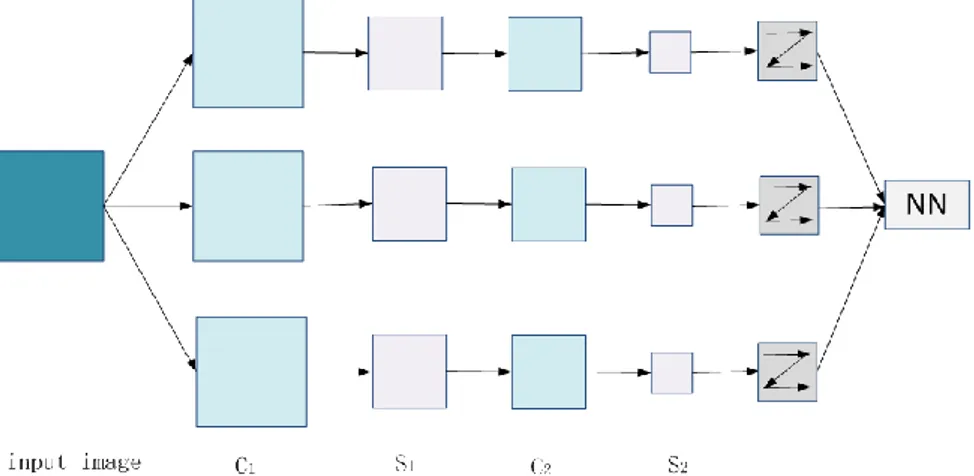
Generally, a CNN takes an overlap structure that consists of several convolutional layers and subsampling layers as its feature extractor, and behind the extractor is a classifier that comprises of a multi-perception structure. Figure 1 shows the structure of a simple CNN model, which is made of two convolutional layers (C1 and C2) and two subsampling layers (S1 and S2). Through making convolutional calculation with three convolutional kernels, the original image generates three feature maps on layer C1. After subsampling, three new feature maps are generated on layer S1, which is then calculated with the three convolutional kernels to
generate three feature maps on layer C2. Subsampling again, three feature maps are generated on layer S2. The three outputs on S2 are vectored, then inputted and trained in a conventional neural network.
As can be seen from the structure of CNN, features are extracted through convolutional layers, and the dimensions of the features are reduced through subsampling. The features are then converted into more abstract ones that can be used to represent the image.
Figure 1. Structure of convolutional neural network
2.3. CNN Training Algorithms
Like the training algorithms of a conventional back propagation (BP), the CNN training algorithms include forward transmission and backward transmission.
1) In the forward transmission stage, a sample (X Oi, i) is picked out from the sample
set and inputted into the network, in which, the sample is transferred layer-by-layer and transmitted to the output layer. The practical output
O
i can be calculated according to relation (1): (1) (1) (2) (2) ( ) ( ) 1 2 1(
(
( (
)
) )
n n i n n iO
F F
F F X w
b
w
b
w
b
(1)where, Fn( ) is the activation of layer n;
( )n
w
is the weight of layer n;b
( )n is the bias of layer n. 2) In the backward transmission stage, the difference between the practical outputi O
and the ideal output Yi is calculated, which is then used to adjust the weight matrix by using the minimum error method. In this stage, there are the reversed error transmission on the output layer and the reversed error transmission on the hidden layer. The error during the reversed error transmission on the output layer can be calculated according to (2) and (3), as follows:
2 1 ( ) 2 i k ik ik E
O T (2) i ik ik ikE
O
T
O
(3) where, Ei, Oik and Tik are the error of sample i, the output of neuron k of sample i on the output layer, and the expected output of neuron k of sample i on the output layer, respectively.The errors can be transmitted either on the subsampling layer or on the convolutional layer. The method to calculate the error on the subsampling layer is similar to the method to calculate the error on the output layer, while the calculation of the error transmission on the convolutional layer is much complex, which, in most case, is solved by using the method [15].
3. The CNN Structure of Crop Pests Image
3.1. Classification of Crop Pests Image Based on LeNet-5
LeNet-5 is a typical CNN structure proposed by LeCun, et al., [16] in 1998, which has been applied to classify handwriting fonts. As shown in Figure 2, a LeNet-5 model contains 5 layers, including 2 convolutional layers, 2 full-connection layers and 1 output layer. If a 32×32 image of handwriting fonts is inputted, the size of the convolutional kernel is 5×5, and the number of the neurons on the output layer is 10. The crop pests image dataset was built by ourselves, there were 82 pest types and the pest image size was 227×227, When we applied LeNet-5 to classify the crop pests image, we were not able to classify the images as the network was not convergent.
3.2. Classification of Crop Pests Image Based on AlexNet
AlexNet was proposed by Alex Krizhevsky, et al., [17] in 2012. For the first time, the deep learning theory was applied to classify large scale images. AlexNet won the championship of the ImageNet Large Scale Visual Recognition Challenge (ILSVRC), with the accuracy reaching 83.6%, which was far higher than conventional ones. The AlexNet contains 8 layers: the first 5 layers are convolutional layers and the other 3 layers are full-connection layers. 3.3. The CNN Structure of Crop Pests
Experimental results of using, respectively, LeNet-5 and AlexNet to process the same crop pests image dataset have shown that the LeNet-5 network was not convergent while the AlexNet achieved good result. There are two causes for this:
The first is the influence of the size of the convolution kernel, which determines the size of reception field. If the reception field is too large, the features to be extracted will exceed the expression of the kernel; if the field is too small, some effective local features will be missed. In the LeNet-5 network, the size of the convolution kernel is 5×5, which is enough to extract the local features of a 32×32 handwriting font image. However, if using this kernel to make convolution to a 227×227 pest image, the kernel is too small to extract all effective information of the local features. In the AlexNet network, the size of the first kernel is 11×11 and the size of the second one is 5×5, in addition to the other three kernels, of which, the sizes are all 3×3. So, the classification by AlexNet is better than that by LeNet-5.
The second is the influence of the structural depth of the network. LeNet-5 has 2 convolutional layers while AlexNet has 5 convolutional layers. For a handwriting font image, the content is relatively single, so its effective features can be extracted only by using 2 convolutional layers. For a pest image, however, the content that contains farmland background is much complex. Therefore, a deeper network is required to extract high-level features. Deep learning can learn and extract the features of an image layer by layer. By increasing the number of the layers, therefore, it gradually becomes stronger to express the features. On the other hand, the structure of the network will be too complex if there too many layers, which requires more training time and may result in over-fitting.
According to the above analysis, we have redesigned the CNN structure based on the AlexNet network to classify the crop pest images, and experimentally checked parameters of the structure: the DCNN contains 7 layers (including 4 convolutional layers); the size of the first convolutional kernel is 9×9; the size of the second one is 5×5, the sizes of the other kernels are 3×3.
4. Experiment Results and Analysis 4.1. Crop Pests Image Dataset
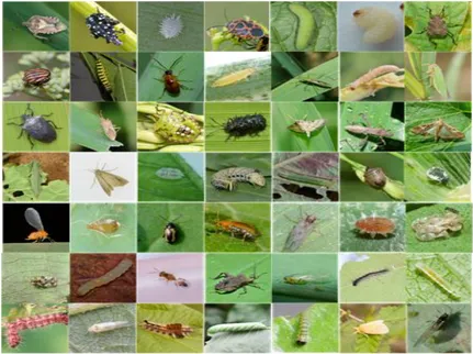
By far, there is no crop pests image dataset that can be commonly used. Therefore, the first thing we have to do is to build a dataset. In our dataset, there are more than 30 thousands images of 82 pest types, including Dolycoris baccarum, Lycorma delicatula, Eurydema and Cicadella viridis. The size of all the images is 227×227, with the format of JPG, and there are about 400 images for each pest type. In the experiment, 300 images of each pest type are taken as the training samples. Figure 2 shows a part number of the pest images that were photographed in the fields.
All the experimental data in this study are sorted, marked and standardized in Economic and Information Research Institute, Anhui Academy of Agricultural Sciences, China and, the
experiment procedure of deep learning is accomplished in the open-source framework Caffe [18].
Figure 2. Part of the field pest image
4.2. Designing the Deep Network Structure 4.2.1. Convolutional Kernel
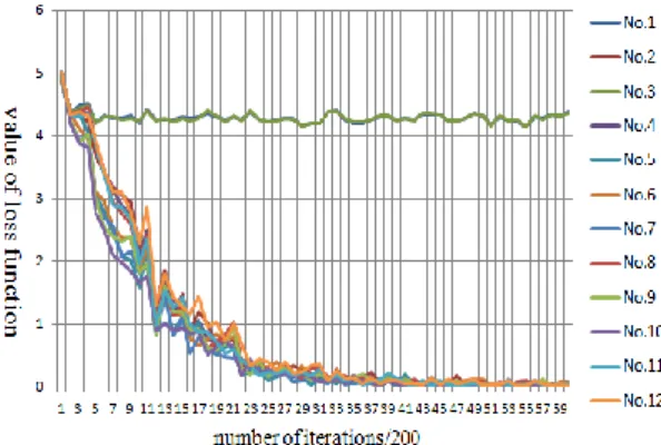
Based on the AlexNet structure with the number of the layers unchanged, we have changed the sizes of the convolutional kernels and designed 12 groups of the kernels. The kernel sizes in each group are listed in the second column of Table 1. The sizes of the feature maps are 96, 256, 384, 384 and 256, respectively; the convolution steps are 4, 1, 1, 1 and 1, respectively, the numbers to complement the convolution borders are 0, 2, 1, 1 and 1, respectively. The classification accuracy of different convolutional kernels is listed in table 1. The value of loss function trained by using different convolutional kernels is shown in Figure 3, of which, the X-axis represents the number of iterations and the Y-axis represents the value of the loss function. Each value is calculated during every 200 iterations. Figure 4 shows the curve of the classification accuracies, in which, the X-axis represents the number of iterations and the Y-axis represents the classification accuracy. The batch size is 64 and the classification accuracy is calculated during every 1000 iterations.
Table 1. Classification accuracy of different convolution kernels No Kernel sizes Classification accuracy
1 7、5、1、1、1 4.33% 2 7、5、3、3、3 88.43% 3 9、5、1、1、1 4.33% 4 9、5、3、3、3 89.63% 5 9、7、3、3、3 88.84% 6 11、9、3、3、3 88.07% 7 11、7、3、3、3 88.43% 8 11、5、3、3、3 88.76% 9 13、11、3、3、3 87.89% 10 13、9、3、3、3 88.42% 11 13、7、3、3、3 88.96% 12 13、5、3、3、3 88.13%
Figure 3. Loss function value curve of different convolution kernels
Figure 4. Classification accuracy curve of different convolution kernels
As can be seen from Table 1, Figure 3 and 4, the networks in experiment 1 and 3 are not convergent. The accuracy of the classification is the highest in experiment 4, in which, the size of the first convolutional kernel is 9; the size of the second one is 5, the sizes of the others are 3.
4.2.2. The Number of Network Layers
Based on the above experimental results, we determine that: the size of the first convolutional kernel is 9; the size of the second one is 5; the sizes of the others are 3, the numbers of the convolutional layers are 3, 4, 6, 7 and 8, with keeping other parameters unchanged. The classification accuracies are listed in Table 2. Figure 4 shows the curve of the training loss function, and Figure 5 shows the curve of the classification accuracies.
Table 2. Classification accuracy of different numbers of convolution layers
No Convolution layers Classification accuracy
13 3 89.02%
14 4 91.00%
15 6 87.95%
16 7 60.59%
17 8 4.33%
Figure 5. Loss function value curve of different numbers of convolution layers
Figure 6. Classification accuracy curve of different numbers of
It can be seen from Table 2, Figure 4 and 5 that: the network in experiment 17 is not convergent. The accuracy (91%) is the highest in experiment 14, in which, the number of the convolutional layers is 4.
4.3. Comparison of the Experimental Results
The accuracy would be low if using SVM or BP to classify pest images in a conventional way, say, pest features (color, shape and texture) are manually designed. Generally, samples will be reprocessed by removing those complex backgrounds in the images to raise the accuracy. In this way, the accuracy can be raised to 80%. However, the reprocessing is tedious and is affected by human subjective consciousness. The accuracy of our method and the conventional ones are compared in Table 3.
Table 3. Comparison between our method and traditional methods
No Methods Classification accuracy
1 Our Method 91%
2 Manually designed features + BP 55%
3 Manually designed features +SVM 60%
4 Removing complex backgrounds + manually designed features+ BP or SVM 80%
Table 3 shows that DCNN can achieve a higher accuracy when compared to conventional classification method, as it is better at extracting pest features.
5. Conclusion
A DCNN-based method was proposed in this study to classify crop pests image. In this method, the classification can be accomplished by using DCNN to extract those complex features, dispensing with an intricate manual extraction. LeNet-5 and AlexNet were applied to classify the crop pest images from dataset that we built by ourselves. The network structure was redesigned by comparing both advantages and disadvantages of the two networks. Our experiment proves that our CNN structure performs well in classifying crop pest images, with the accuracy reaching 91%. In addition, this paper can be taken as a reference of building a deep-network to solve relative problems.
Acknowledgements
This work was supported by the National Natural Science Foundation of China (No.31671586).
References
[1] Z Li, T Hong, X Zeng, et al. Citrus red mite image target identification based on K-means clustering. Transactions of the Chinese Society of Agricultural Engineering. 2012; 28(23): 147-153.
[2] S Huang, Research on the key techniques of image-based insects recognition. XiAn, China: NorthWest University; 2008.
[3] H Zhang, H Mao, D Qiu. Feature extraction for stored-grain insect detection system based on image recognition technology. Transactions of the Chinese Society of Agricultural Engineering. 2009; 25(2): 126-130.
[4] J Wang, C Lin, L Ji, et al. A new automatic identification system of insect images at the order level. Knowledge-Based Systems. 2012; 33: 102-110.
[5] Y Hong, L Song, J Zhang, et al. Pest image recognition of multi-feature fusion based on sparse representation. Pattern Recognition and Artificial Intelligence. 2014; 27(11): 985-992.
[6] C Xie, J Zhang, R Li, et al. Automatic classification for field crop insects via multiple-task sparse representation and multiple-kernel learning. Computers and Electronics in Agriculture. 2015; 119: 123-132.
[7] Z Wen, L Cao. Machine recognition of disease and insect pests on citrus fruits using complexity measurement . Chinese Agricultural Science Bulletin. 2015; 31(10): 187-193.
[8] L Zhu, Z Zhang. Using CART and LLC for image recognition of Lepidoptera. Pan-Pacific Entomologist. 2013; 89(3): 176-186.
process for automating bee species identification based on wing images and digital image processing. Ecological Informatics. 2014.
[10] Hinton G Salakhutdinov R. Reducing the dimensionality of data with neural networks. Science. 2006; 313(5786): 504-507.
[11] Large Scale Visual Recognition Challenge 2012 (ILSVRC2012). 2013.
[12] K Yu, L Jia, Y Chen, et al. Deep learning: yesterday, today, and tomorrow. Journal of Computer Research and Development. 2013; 50(9): 1799-1804.
[13] Z Sun, L Xue, Y Xu, et al. Overview of deep learning. Application Research of Computers. 2012; 29(8): 2806-2810.
[14] Bengio Y. Practical recommendations for gradient-based training of deep architectures. Berlin: Springer-Verlag. 2012: 437-478.
[15] Simard P, Steinkraus D, Piatt JC. Best practices for convolutional neural networks applied to visual document analysis. ICDAR 2003. Scottland. 2003: 958-962.
[16] Y Lecun, L Bottou, Y Bengio, et al. Gradient-based earning applied to document recognition. Proceedings of the IEEE. 1998.
[17] A Krizhevsky, I Sutskever, G Hinton. Imagenet classification with deep convolutional neural networks. Conference and Workshop on Neural Information Processing Systems. 2012.
[18] Y Jia, Evan Shelhamer, Jeff Donahue, et al. Caffe: Convolutional Architecture for Fast Feature Embedding. Computer Vision and Pattern Recognition. 2014.