COX, CRAIG ALLEN. Development and Flight Test of a Multi-Function Controller for Automated Cruise Flaps on an Aircraft Wing. (Under the direction of Charles E. Hall, Jr. and Ashok Gopalarathnam.)
Cruise flaps are trailing-edge flaps which minimize the profile drag of a wing by moving the low-drag-region (or bucket) of a drag polar such that it spans the current coefficient of lift. Previous research has explored the use of a pressure-based technique for automating cruise flaps. Data obtained using this technique can be presented in a number of different formats, and different presentations of the same data tend to lead to the development of different types of automating controllers. The presentation used by previous researchers led to the development of a drag-minimizing controller that required a low-pass filter to prevent instability. This prevented the controller from being used for purposes which required a fast-acting flap. The presentation of pressure data used in this research led to the development of a multi-function controller that includes both slow-acting functionality (drag reduction) and fast-acting functionality (gust alleviation).
The pressure-based technique developed by previous researchers using natural-laminar-flow (NLF) airfoils must be modified somewhat for the low Reynolds number SD7037 airfoil used in this research. Drag polars for low Reynolds number airfoils do not behave as predictably as those for NLF airfoils at much higher Reynolds numbers. A series of rigid-aircraft simulations were conducted to show the effectiveness of the multi-function controller, which was able to simultaneously reduce drag and alleviate the effects of vertical gusts.
by
Craig Allen Cox
A dissertation submitted to the Graduate Faculty of North Carolina State University
in partial fulfillment of the requirements for the Degree of
Doctor of Philosophy
Aerospace Engineering
Raleigh, North Carolina
2008
APPROVED BY:
Dr. Paul Ro Dr. Pierre Gremaud
Dr. Ashok Gopalarathnam Dr. Charles E. Hall, Jr.
DEDICATION
This dissertation is dedicated to the members of my immediate family: my wife Regina and our children Alec and Erin.
Regina, you have always supported me in my decision to go back to school late in life. You knew that there were financial and other costs that might never be made up, but you understood my need to do this. We may be an old married couple, but you should never underestimate how important you are to me and how much I depend on you. You helped turn me from who I was to who I am, and everyone thanks you for that.
Alec and Erin, you have both made us so proud over the years and continue to do so. You are wonderful children and have always been so. I have spent a lot of time over the last six years on my studies and research, and that is time that was taken from you. I am sorry for that. If it is any consolation, one of the reasons that I was able to devote time to my education is because you are the young man and young woman that you are. You are thoughtful, well-behaved, and most importantly, have a great deal of empathy for others. We never had to worry about either of you, and it is doubtful that we ever will.
Erin and Alec, in a few short years you will both have left the nest and struck out on your own in this world. There is a lot of advice I could give you, but you have probably already figured out the important stuff. One thing I will repeat. No matter how you choose to make your living, think like a scientist. Be open-minded, objective, and impartial. Most importantly...
BIOGRAPHY
Craig Allen Cox was born in Lapeer, Michigan, on June 15, 1961, to Homer Elwin Cox and Charlotte June McCready Cox. His family moved to Pikeville, Kentucky, when he was eight years old, and he lived there until he graduated from Millard High School in 1979. He worked for one year before attending one year at the University of Kentucky at Lexington. He then attended the U.S. Naval Academy in Annapolis, Maryland. He graduated in 1985 with a Bachelor of Science in Applied Science (Computer Track).
While serving in the U.S. Navy, Craig attended The George Washington Univer-sity in Washington, D.C. He obtained a Master of Science in Computer Science (Artificial Intelligence) in 1993. After his naval service ended in 1993, he worked as a contract software developer for numerous companies.
ACKNOWLEDGEMENTS
I would first like to acknowledge the members of my committee. Dr. Hall for his assistance with hardware and software issues, and for bringing me into flight test environ-ments where I learned things that were invaluable for this research. Dr. Gopalarathnam for his guidance and ability to explain aerodynamic concepts so that even I can understand them. Dr. Ro for being an outstanding instructor in the SISO and MIMO classes where I learned 90% of what I know about controls. Dr. Gremaud for forcing me to relearn differ-ential equations after they had left my brain 15 years ago. Like Dr. Hall said, “How do you expect to be able to do controls if you can’t do differential equations?”
This research and my continuing education would not have been possible without the very generous support of Dr. Donald Moreland and his wife Verdie Moreland. They established the Frank C. Ziglar, Jr. Endowed Graduate Fellowship, which provided support to my family for two years. It is no exaggeration to say that without this support I could not have completed this phase of my education. Donald and Verdie, I am indebted to you and you should never underestimate the effect of your generosity. Thank you.
KalScott Engineering also supported this research through a Phase-2 STTR project from the NASA Dryden Research Center. Their contribution enabled this research to con-tinue up through flight testing, which was one of the most enjoyable (and nerve-wracking) aspects of the research.
Air Force Research Laboratory (AFRL) supported me during my educational pur-suit through their co-operative education program with North Carolina State University. During my years of study, I worked at Wright-Patterson Air Force Base over four co-op sessions at the Control Systems Development and Applications Branch, and the Aerody-namic Configuration Branch. This work was the determining factor in my choice of AFRL for post-graduate employment.
A general thank you to the worldwide Linux community, whose contributions allowed me to conduct this research using an operating system that I find much more intuitive and easier to navigate than the alternative. But then again, I am a “vi” kind of guy.
http://gputils.sourceforge.net. GPUTILS is an outstanding suite of utilities for working with PIC microcontrollers from Microchip Technology, Inc. It includes thegpasmassembler used to develop code for this research. Orion Sky Lawlor is the author of the excellent usb pickitutility for writing compiled code to PIC microcontrollers. His development of this utility and its contribution to the open-source community meant that this research could be done 100% in Linux without having to switch operating systems to talk to the microcontrollers.
Flight testing isn’t always fun, but there were always people willing to help out. Adam Propst was the pilot for the first two flight test days, and Stearns Heinzen piloted the last two days. Jason Bishop and Dave Burke helped out with ground duties, and their willingness to assist was invaluable.
Thank you to Stearns Heinzen, a wealth of information and the go-to person when you need someone to talk through your good ideas and shoot down your bad ideas before they can waste your time. He is a large part of the corporate knowledge of the aerospace engineering department, and a very good friend.
I will miss everyone in the Langley room lunch group and the political discussions we had. The only annoying part was when the need to get some actual work done interfered with our primary task of deciding how to save the world (whether it wanted it or not).
TABLE OF CONTENTS
LIST OF FIGURES . . . viii
NOMENCLATURE . . . xiii
1 Introduction . . . 1
1.1 Overview . . . 1
1.2 Background . . . 1
1.3 Objectives . . . 7
1.4 Overview of Dissertation Chapters . . . 8
2 Analysis and Simulation . . . 10
2.1 Overview . . . 10
2.2 Analysis of Previous Control Scheme . . . 10
2.3 Simulation Model . . . 16
2.4 Coefficient Determination . . . 22
2.5 Controller Functions . . . 26
2.6 Controller Performance . . . 29
3 Controller Hardware/Software . . . 38
3.1 Overview . . . 38
3.2 General Information . . . 38
3.3 Communications Scheme . . . 40
3.4 DCPP Reader . . . 44
3.5 Servo Reader . . . 49
3.6 Servo Writer . . . 53
3.7 Servo Calculator . . . 58
3.8 Fail-Safe Switch . . . 72
4 Analysis of Flight Test Results . . . 74
4.1 Overview . . . 74
4.2 General Information . . . 74
4.3 Test of Initial ∆C′ p-Measurement System . . . 76
4.4 Test of Expanded-Scale ∆C′ p-Measurement System . . . 79
4.5 Test of ∆C′ p-Maintenance Function . . . 90
4.6 Test of ∆C′ p-Optimization Function . . . 100
5 Conclusions and Future Work. . . 115
5.1 Overview . . . 115
5.2 Conclusions . . . 115
5.3 Future Work . . . 118
APPENDICES . . . 123
A Data Overviews for Flights Testing the Expanded-Scale∆C′
p-Measurement
System . . . 124
B Data Overviews for Flights Testing the ∆C′
p-Maintenance Function . . . 133
C Data Overviews for Flights Testing the ∆C′
LIST OF FIGURES
Figure 1.1 Comparison of maximum thickness locations and laminar-to-turbulent tran-sitions for NACA 4415 and NLF(1)-0215F airfoils at a Reynolds number of 6×10⁶. 2 Figure 1.2 Comparison of drag polars for NACA 4415 and NLF(1)-0215F airfoils at a
Reynolds number of 6×10⁶. . . . 3
Figure 1.3 Shift of drag bucket with flap deflection. . . 4
Figure 1.4 Ideal stagnation-point range. . . 5
Figure 1.5 Pressure port locations.. . . 6
Figure 2.1 ∆C′ p as a function of Cl for different flap angles. . . 11
Figure 2.2 Cl-αcurves for different flap angles illustrating the behavior of an unstable flap controller. . . 13
Figure 2.3 ∆C′ p as a function of α for different flap angles. . . 14
Figure 2.4 Cl-αcurves for different flap angles illustrating the behavior of a stable flap controller. . . 15
Figure 2.5 AVL model of the Spirit 100 sailplane. . . 17
Figure 2.6 SD7037 drag polars with optimalCl values. . . 18
Figure 2.7 ∆C′ p-Cl curves showing optimal Cl values for the SD7037. . . 19
Figure 2.8 Constant ∆C′ p value of −1.85 for the SD7037. . . 20
Figure 2.9 Drag polars for ∆C′ p target of −1.85 for the SD7037.. . . 21
Figure 2.10 ∆C′ p-δf linear fit for wing lift coefficient of 0.78. . . 23
Figure 2.11 δf-Cl linear fit for ∆Cp′ =−1.85. . . 24
Figure 2.12 Partial gust-alleviation function. . . 26
Figure 2.13 ∆C′ p-optimization function. . . 27
Figure 2.14 ∆C′ p-maintenance function. . . 28
Figure 2.16 Gust profile. . . 30 Figure 2.17 Gust-alleviation performance.. . . 33 Figure 2.18 ∆C′
p-optimization performance. . . 34 Figure 2.19 ∆C′
p-maintenance performance. . . 35 Figure 2.20 ∆C′
p-optimization and maintenance performance. . . 36 Figure 2.21 Full control performance. . . 37
Figure 3.1 XFOIL data showing the leading-edge pressure differential that can be expected in flight. . . 44 Figure 3.2 XFOIL data showing the mid-chord pressure differential that can be
ex-pected in flight. . . 45 Figure 3.3 Calibration curve for the±1 inch differential pressure transducers. . . 46 Figure 3.4 Calibration curve for the 0–1 inch gauge pressure transducers. . . 47 Figure 3.5 Calibration curve for flaps showing the relationship between servo pulse
width and surface deflection angle. . . 54 Figure 3.6 Calibration curve for ailerons showing the relationship between servo pulse
width and surface deflection angle. . . 55 Figure 3.7 Calibration curve for elevator showing the relationship between servo pulse
width and surface deflection angle. . . 59 Figure 3.8 Test ∆C′
pvalues used to compare the performance of a first-order PI control block and that of a second-order PID control block. . . 61 Figure 3.9 Comparison of the output of the full PID, exact PI, and simplified PI
blocks.. . . 63 Figure 3.10 State variable values obtained during tests of different PI control blocks. . 66
Figure 4.1 Photo of the Spirit 100 with Stearns Heinzen (pilot), Adam Propst (pilot), Craig Cox (author), Jason Bishop (ground crew), and Dave Burke (ground crew). 75 Figure 4.2 ∆C′
p values for flight 1 (full-scale). . . 77 Figure 4.3 ∆C′
Figure 4.4 Discretization of filtered ∆C′
p error for flight 1. . . 79 Figure 4.5 ∆C′
p values for flights 4–7. . . 80 Figure 4.6 Discretization of filtered ∆C′
p error for flight 5. . . 81 Figure 4.7 Comparison of zero-flap raw ∆C′
p data with XFOIL prediction for flights 2, 3, 4, and 7.. . . 83 Figure 4.8 Transition curves for an SD7037 airfoil with ∆C′
p drop-off marked. . . 84 Figure 4.9 Comparison of zero-flap smoothed ∆C′
p data with XFOIL prediction for flights 2, 3, 4, and 7. . . 86 Figure 4.10 Illustration of the effect of a central moving-average filter on data outliers. 87 Figure 4.11 Time history of ∆C′
p data showing groups of at least 5 and groups of at least 10. . . 88 Figure 4.12 Comparison of XFOIL prediction with experimental data showing groups
of at least 5 and groups of at least 10. . . 89 Figure 4.13 Results of ∆C′
p-maintenance function for flight 17. . . 91 Figure 4.14 Flight 16 CL and ∆Cp′ data showing periods of no elevator deflection. . . 92 Figure 4.15 Flight 16CLand ∆Cp′ data highlighting data points from 19 to 21 seconds. 94 Figure 4.16 Least-squares fit ofCL and ∆Cp′ data for periods of flights 16 and 18 with
no elevator movement.. . . 95 Figure 4.17 Least-squares fit of CL and ∆Cp′ data for periods of flight 19 with no
elevator movement.. . . 96 Figure 4.18 Residual ∆C′
p for a portion of uncontrolled flight 16. . . 98 Figure 4.19 Residual ∆C′
p for a portion of controlled flight 19. . . 99 Figure 4.20 Smoothed, filtered, and target ∆C′
p values for flight 21. . . 102 Figure 4.21 Pilot-commanded and controller-generated surface deflections for flight 21.103 Figure 4.22 Filtered ∆C′
p error and optimizing flap for flight 21. . . 104 Figure 4.23 Least-squares fit of filtered ∆C′
p error and optimizing flap for flight 21.. . . 105 Figure 4.24 Smoothed, filtered, and target ∆C′
Figure 4.25 Smoothed, filtered, and target ∆C′
p values for flight 23. . . 107
Figure 4.26 Smoothed, filtered, and target ∆C′ p values for flight 24. . . 108
Figure 4.27 Smoothed, filtered, and target ∆C′ p values for flight 25. . . 109
Figure 4.28 Pilot-commanded and controller-generated surface deflections for flight 25.111 Figure 4.29 Smoothed, filtered, and target ∆C′ p values for flight 26. . . 112
Figure 4.30 Smoothed, filtered, and target ∆C′ p values for flight 27. . . 113
Figure A.1 Data overview for flight test 2.. . . 125
Figure A.2 Data overview for flight test 3.. . . 126
Figure A.3 Data overview for flight test 4.. . . 127
Figure A.4 Data overview for flight test 5.. . . 128
Figure A.5 Data overview for flight test 6.. . . 129
Figure A.6 Data overview for flight test 7.. . . 130
Figure A.7 Data overview for flight test 8.. . . 131
Figure A.8 Data overview for flight test 9.. . . 132
Figure B.1 Data overview for flight test 10. . . 134
Figure B.2 Data overview for flight test 11. . . 135
Figure B.3 Data overview for flight test 12. . . 136
Figure B.4 Data overview for flight test 13. . . 137
Figure B.5 Data overview for flight test 14. . . 138
Figure B.6 Data overview for flight test 15. . . 139
Figure B.7 Data overview for flight test 16. . . 140
Figure B.8 Data overview for flight test 17. . . 141
Figure B.9 Data overview for flight test 18. . . 142
Figure B.11 Data overview for flight test 20. . . 144
Figure C.1 Data overview for flight test 21. . . 146
Figure C.2 Data overview for flight test 22. . . 147
Figure C.3 Data overview for flight test 23. . . 148
Figure C.4 Data overview for flight test 24. . . 149
Figure C.5 Data overview for flight test 25. . . 150
Figure C.6 Data overview for flight test 26. . . 151
NOMENCLATURE
CL aircraft lift coefficient
CLw wing lift coefficient
CLα change in aircraft lift due to angle of attack
CLα˙ change in aircraft lift due to derivative of angle of attack
CLα,w change in wing lift due to angle of attack
CLδe change in aircraft lift due to elevator deflection
CLδf change in aircraft lift due to flap deflection
CL˙
δf change in aircraft lift due to derivative of flap deflection
CLδf ,w change in wing lift due to flap deflection
Cd airfoil drag coefficient
Cl airfoil lift coefficient
Cm aircraft pitching moment coefficient
Cmα change in aircraft pitching moment due to angle of attack
Cmα˙ change in aircraft pitching moment due to derivative of angle of
attack
Cmδe change in aircraft pitching moment due to elevator deflection
Cmδf change in aircraft pitching moment due to flap deflection
Cmδf˙ change in aircraft pitching moment due to derivative of flap
deflec-tion
GC(s) transfer function for the PID or PI controller that implements
GF(s) transfer function for the low-pass filter that processes pressure-differential error
I0 4-line multiplexer input which receives pilot-commanded servo
pulses from the radio-control (R/C) receiver
I1 4-line multiplexer input which receives servo pulses generated by
the on-board controller
KD derivative gain
KI integral gain
KP proportional gain
Re Reynolds number
S multiplexer selector line which determines whether the servo pulses
output are those from the radio-control receiver or those from the on-board controller
(dCL/dδe)Cm=0 change in trim aircraft lift due to elevator deflection
(dCLw/dδe)Cm=0 change in trim wing lift due to elevator deflection
(dCLw/dδf)∆C′
p=const change in wing lift at constant pressure differential due to flap
deflection
(dδe/dCL)∆C′
p=const change in elevator required for trim aircraft lift change at constant
pressure differential
dδe/d∆Cp′
CLw=const pressure-differential-to-elevator ratio for constant wing lift (dδe/dδf)C
Lw=const flap-to-elevator mixing ratio for constant trim wing lift
(dδf/dCL)∆C′
p=const change in flap required for trim aircraft lift change at constant
pressure differential
dδf/d∆Cp′
CLw=const pressure-differential-to-flap ratio for constant wing lift
pl,l leading-edge lower surface pressure
pl,u leading-edge upper surface pressure
pu mid-chord upper surface pressure
s variable used in the Laplace transform representation of control
system transfer functions
un input vector for the current time step in a discrete-time state-space representation
xn state vector for the current time step in a discrete-time state-space representation
xn+1 state vector for the next time step in a discrete-time state-space representation
yn output vector for the current time step in a discrete-time
state-space representation
∆CL incremental aircraft lift coefficient
∆CLw incremental wing lift coefficient
∆Cm incremental aircraft pitching moment
∆C′
p ratio of leading-edge pressure differential to absolute value of mid-chord pressure differential
∆α incremental angle of attack
∆δe incremental elevator deflection
∆δf incremental flap deflection
α angle of attack
˙
α derivative of angle of attack
δe elevator deflection angle
δec commanded elevator deflection angle
δf flap deflection angle
˙
δf derivative of flap deflection angle
γ temporary variable
Chapter 1
Introduction
1.1
Overview
This chapter presents background information on natural-laminar-flow airfoils and cruise flaps. It introduces earlier research on automation of cruise flaps using a pressure-based technique. It lists the objectives of this research, and provides an overview of disser-tation chapters and how they address the objectives.
1.2
Background
Airflow past an airfoil will begin as laminar flow and will transition at some point to turbulent flow. Since turbulent flow results in more drag due to skin friction, it is generally desirable to maintain laminar flow for as long as possible. The point at which laminar flow transitions to turbulent flow on the upper or lower surface of an airfoil is affected by the point of maximum local velocity, which is related to the point of maximum airfoil thickness (for small angles of attack). In areas of increasing local velocity, the pressure gradient is favorable and flow tends to stay laminar. When local velocity begins to decrease, the pressure gradient becomes adverse and laminar flow is more likely to become turbulent.
Figure 1.1: Comparison of maximum thickness locations and laminar-to-turbulent transi-tions for NACA 4415 and NLF(1)-0215F airfoils at a Reynolds number of 6×10⁶.
number (Re) of 6×10⁶. The NLF airfoil has its minimum drag at aC
l of approximately 0.65, so the laminar-to-turbulent transition points for thisCl were found for the upper and lower surfaces. For the NACA 4415, these transitions occurred at 42% and 30% of chord, respectively. For the NLF(1)-0215F, transitions occurred at 55% and 64%. The percentage of laminar flow for the NACA 4415 is approximately 36%, while the NLF(1)-0215F has almost 60% laminar flow. This is one reason that the NLF airfoil has lower drag at this Cl (0.0042 compared to 0.0059).
Figure 1.2: Comparison of drag polars for NACA 4415 and NLF(1)-0215F airfoils at a Reynolds number of 6×10⁶.
when operated at Cl values for which they were designed, but this advantage is lost (and sometimes reversed) at off-design values of Cl.
Figure 1.3: Shift of drag bucket with flap deflection.
cruise flap, when scheduled correctly, can result in a large range ofClvalues over which low
Cd is achieved. For this reason, several NLF airfoils have been designed with cruise flaps [4, 5, 6]. Cruise flaps have also been successfully used on high-performance sailplanes for several decades.
Figure 1.4: Ideal stagnation-point range.
Figure 1.5: Pressure port locations.
is unaffected by dynamic pressure. Numerically, taking a ratio of pressures measured in flight is identical to taking a ratio of pressure coefficients calculated using tools like XFOIL. Vosburg and Gopalarathnam [8] noted that an airfoil with an automated cruise flap has lift and moment curves with unusual characteristics. While a normal lift curve has a nearly constant slope approximating 2π/rad, the automated cruise flap lift curve has three distinct areas. At low Cl values the flap is held constant at some negative deflection limit, either a physical limit based on flap geometry or some other limit determined by how much physical travel is desired when the flap is actuated as a cruise flap. At these low Cl values with a constant flap deflection, the lift curve slope is approximately 2π/rad. At high Cl values the flap is held constant at some positive deflection limit, and the lift curve slope is again approximately 2π/rad. Between these two Cl limits, though, the flap angle changes asCl changes, and the result is a lift curve with a negative slope. In this Cl range where cruise flap motion occurs, a desired increase inCl actually requires that angle of attack be decreased. The moment curve for an airfoil with an automated cruise flap is also unusual. Normally, pitching moment about the quarter-chord is not affected much by changes in angle of attack (or Cl). With an automated cruise flap, though, changes in
Cl result in changes in flap deflection, which cause large (and predictable) changes in the pitching moment.
flaps. They examined the response of an aircraft with an automated cruise flap which was controlled using the instantaneous coefficient of lift as the sole input. Such a flap, by itself, was found to be unstable. From a trimmed state, if the wing were perturbed such that the coefficient of lift were increased, the flap angle would increase to move the stagnation point back to the ideal location. The larger flap angle would then increase the coefficient of lift even more, and the flap would quickly diverge to its limit of travel. Although aircraft such as uninhabited air vehicles (UAVs) are probably equipped with separate autopilot control systems to maintain altitude and airspeed, such systems could not counter the instability of the flap controller since the flap system has such a short time constant (determined primarily by the reaction time of the flap servo). A filter is needed to slow the operation of the flap.
Cox, Gopalarathnam, and Hall [9] performed a dynamic stability analysis of the Vosburg and Gopalarathnam controller to examine the source of the instability. They showed that the aircraft without automated cruise flaps has negative real parts for all of its eigenvalues (i.e., the aircraft is stable). Implementation of an automated cruise flap adds a positive real eigenvalue, which results in monotonic instability. The time-to-double is a factor of the flap servo responsiveness, with faster servos making the problem worse by decreasing the time it takes to drive the servo to its limit.
Cox, Gopalarathnam, and Hall [9] also examined the Vosburg and Gopalarath-nam controller to show its behavior under different operating conditions and with different slowing filters. They developed an aircraft controller to maintain a desired coefficient of lift using flap deflections. This type of controller will likely be useful in future research with segmented flaps for tailoring the span-wise lift distribution to minimize induced drag or wing root bending moment.
1.3
Objectives
presents the development of an improved, multi-function flap controller, and culminates in flight testing of a radio-controlled (R/C) aircraft with automated cruise flaps.
The objectives of this research were to:
1. Conduct a more in-depth exploration of the stability and control issues of an aircraft with automated cruise flaps.
2. Develop a multi-function controller with both slow-acting functionality (drag reduc-tion) and fast-acting functionality (gust alleviareduc-tion).
3. Conduct simulations in Simulink to assess the performance of all functions of the controller.
4. Develop the hardware and software required to implement a flight-ready controller using low-cost microcontrollers and transducers.
5. Conduct flight tests using an R/C glider to assess the performance of the slow-acting functionality of the controller.
1.4
Overview of Dissertation Chapters
This section presents an overview of the chapters of this dissertation and shows how the chapter topics address the objectives of the research.
Chapter 2 examines previous research on pressure-based methods for automating cruise flaps and shows how different methods of presenting pressure data tend to lead to the development of different types of controllers. It details the development of a new multi-function controller which provides both drag reduction and gust alleviation. Finally, it displays and discusses the results of simulations that examine the performance of this controller under various conditions. This chapter addresses objectives 1–3.
Chapter 3 presents the details of the hardware and software which were used to implement the flight-ready automated cruise flap controller. It discusses how controller functionality is broken down into simple tasks that can be executed by one of five separate modules. It also explains the communication scheme that was developed to allow data to be passed from one module to another. This chapter addresses objective 4.
controller. For most sets the results confirmed the correct operation of the controller; for one set the data were inconclusive. This chapter addresses objective 5.
Chapter 2
Analysis and Simulation
2.1
Overview
This chapter examines previous research on pressure-based methods for automat-ing cruise flaps and shows how different methods of presentautomat-ing pressure data tend to lead to the development of different types of controllers. It details the development of a new multi-function controller which provides both drag reduction and gust alleviation. Finally, it displays and discusses the results of simulations that examine the performance of this controller under various conditions.
2.2
Analysis of Previous Control Scheme
The ratio of leading edge pressure differential to mid-chord differential is given by the following equation, where the pressures are measured at the locations shown in Fig. 1.5.
∆C′
p =
pl,u−pl,l
|pu−pl|
For NLF airfoils with a range of flap deflections, a target ∆C′
p can be selected. If the airfoil is operated at or near this target, it is guaranteed to be operating in the low-drag region regardless of flap angle or lift coefficient. Operations at other than the target ∆C′
p result in an error, either negative (actual ∆C′
there are two obvious choices: increase or decrease flap deflection. The choice of presentation of the ∆C′
p data for different flap angles affects the controllers that are developed.
Figure 2.1: ∆C′
p as a function of Cl for different flap angles.
The paper by McAvoy and Gopalarathnam [7] included figures similar to Fig. 2.1, which shows ∆C′
p as a function of Cl on the horizontal axis for the NASA NLF(1)-0215F airfoil [5]. For each flap curve, filled and unfilled circles mark the bottom and top, respec-tively, of the drag bucket for that flap angle. Asterisks mark a target point which is 0.05
Cl above the bottom of the drag bucket. Although the bottom of the drag bucket is where minimum drag occurs for this airfoil, it is also the location of a corner in the drag polar where a slight decrease inClresults in a large increase in drag. Setting the target point 0.05
Cl higher than the bottom of the drag bucket prevents small deviations about the target ∆C′
Since the target ∆C′
p values for all flap curves in Fig. 2.1 are close to −0.37, this value is chosen as the target value that a controller must try to maintain. Assume that an airfoil is operating in steady-state conditions with a flap angle of−8 deg at location A. There is no ∆C′
p error so the flap does not move. A gust occurs such that Cl increases by about 0.2. Since the flap has not yet changed, the operating condition moves along the−8 deg flap curve to location B. This changes ∆C′
p from −0.37 to about −1.25, resulting in a negative error. This particular presentation of the ∆C′
p data makes it appear that the correct response is to increase flap to move along the constant-Cl line to location C. Here the flap value is−2 deg and ∆C′
p returns to the target value of−0.37. This presentation of the ∆C′
p data tends to lead to the development of the following rule: “To fix a non-optimal condition, determine the optimal flap value for the current Cl and move the flap toward that value.” From Fig. 2.1, this implies that correction of a negative ∆C′
p error requires that flap be increased, so there is a negative correlation between ∆C′
p error and corrective flap movement.
The paper by Vosburg and Gopalarathnam [8] included a figure similar to Fig. 2.2. It was used to demonstrate why a flap controller based on the above rule is unstable. The points A, B, and C correspond to the same points in Fig. 2.1. An airfoil in steady-state conditions at point A experiences a gust which increasesClby 0.2. The operating condition moves along the−8 deg flap curve to point B, which has aCl of about 0.65. This condition is not optimal, so the controller determines the optimal flap angle for a Cl of 0.65 to be−2 deg. The flap is increased from −8 deg to −2 deg, but this change does not occur along a constant-Cl line as expected because a change in flap angle results in a change in airfoil lift. Assuming that the flap can actuate faster than the angle of attack can change, the operating condition moves along a line of constant alpha. The curves in Fig. 2.1 made it appear that the transition from location B would be to location C, but Fig. 2.2 makes it clear that the transition will instead be to location D. The optimality of location D is even worse than that of location B and in the same direction, so the flap is unstable and will quickly diverge to its upper limit.
Figure 2.2: Cl-α curves for different flap angles illustrating the behavior of an unstable flap controller.
either its input (∆C′
p) or output (commanded flap angle) through a low-pass filter. Use of such a filter (or any other slowing mechanism) makes this controller unsuitable for purposes where a fast-acting flap is desired, like gust alleviation.
When presenting ∆C′
p data for different flap angles, using Cl as the horizontal axis makes it easy to answer the question: “What flap angle is required to achieve a target ∆C′
p for the current Cl?” This question, in turn, tends to lead to the development of an unstable controller that is unsuitable for use when a fast-acting flap is desired. But there is at least one other presentation of the data that answers another question and leads to a stable controller.
The important information that Fig. 2.1 provides is that there is a target ∆C′
Figure 2.3: ∆C′
p as a function ofα for different flap angles.
regardless of flap angle in the region of interest from about−10 to 0 deg. By usingClas the horizontal axis, Fig. 2.1 makes it clear that this is also true regardless of Cl in the region of interest from about 0.35 to 0.65. Since it is true regardless of Cl, it must also be true regardless of angle of attack in an appropriate region of interest. This is made clear in Fig. 2.3, which presents the ∆C′
p data with α as the horizontal axis. The target ∆Cp′ values shown in this figure, of course, are also approximately −0.37, so this is the value that a controller must attempt to maintain.
changes ∆C′
p from −0.37 to about −1.0, resulting in a negative error. In this presentation of the ∆C′
p data it appears that the correct response is to decrease flap to move along the constant-α line to location A. Here the flap value is −8 deg and ∆C′
p is again the target value of −0.37. This presentation of the ∆C′
p data tends to lead to development of the following rule: “To fix a non-optimal condition, determine the optimal flap value for the currentα and move the flap toward that value.” From Fig. 2.3, this implies that correction of a negative ∆C′
p error requires that flap be decreased, so there is a positive correlation between ∆C′
p error and corrective flap movement.
Figure 2.4: Cl-α curves for different flap angles illustrating the behavior of a stable flap controller.
curve to point E. This condition is not optimal, so the controller determines the optimal flap angle for anαof about 2.2 deg to be−8 deg. The flap is decreased from−2 deg to−8 deg, and this change occurs along a constant-α line because the flap is assumed to actuate faster than the angle of attack can change. Thus, the operating condition transitions from point E to point A, as was previously indicated in Fig. 2.3. The new location A is optimal, so there is no further flap change and the controller is stable. Two equally valid presentations of the ∆C′
p data steer the development of different controllers. Figure 2.1 leads to a thought process that results in an unstable controller that requires a slowing filter; Fig. 2.3 results in a stable fast-acting controller that can also be used for purposes such as gust alleviation. It should be noted that the simple controller illustrated in Fig. 2.4 is not appro-priate for use without modification. After Cl, α, and ∆Cp′ are perturbed by a gust, the stable response restoring the target ∆C′
p results in an overshoot of the original Cl. The final value ofClis lower than the original, even though the effect of the gust was to increase
Cl. Nevertheless, this simple controller points the way towards the development of a multi-function controller for cruise flap automation. The advantages of three different controllers are combined to result in a cruise-flap controller with three functions: gust alleviation, ∆C′
p optimization, and ∆Cp′ maintenance. The gust-alleviation function is fast acting and uses a positive error/correction correlation to maintain currentCl. The ∆Cp′-optimization function is slow acting and uses a negative error/correction correlation to drive ∆C′
p to a target value which decreases drag. The ∆C′
p-maintenance function is fast acting and uses flap/elevator mixing to maintain current ∆C′
p in the presence of pilot input from the stick or yoke.
2.3
Simulation Model
are trailing-edge down, and positive aileron deflections are trailing-edge down on the right wing.
Figure 2.5: AVL model of the Spirit 100 sailplane.
The AeroSim blockset includes a script used to determine trim values for Simulink models of powered aircraft. This script was modified for use with gliders such as the Spirit 100. References to throttle and engine speed were removed, and the ability to specify a constant descent rate was added. The modified script was used to determine trim values for a number of different descent rates from 0.36 m/s to 0.70 m/s. These descent rates correspond to trim CLvalues from 1.04 to 0.40, respectively. The simulations described in this chapter were performed using the case where the trim descent rate and CL are 0.40 m/s and 0.78, respectively.
The stability derivatives obtained from AVL include terms forδf, but not terms for ˙δf. Since the controller to be developed will activate the flap very quickly for gust alleviation, it was determined that ˙δf derivatives should be implemented in the model. In theory, the effect of ˙δf on aircraft lift and pitching moment should be proportional to the effect of ˙α. Since the effect of flap is to change the airfoil angle at which zero lift is produced (α0L), the aircraft should not be able to distinguish between effects due to ˙α and those due to ˙δf. The ratio of change in α0L to change in δf is the flap effectiveness parameter τf, so the following are the calculated ˙δf derivatives.
CLδf˙ =CLα˙τf
Cmδf˙ =Cmα˙τf
Earlier research regarding ∆C′
million, for example, that McAvoy and Gopalarathnam [7] first discovered that constant-∆C′
p operations occur in the drag bucket for the NLF(1)-0215F and NLF(1)-0414F airfoils. Drag polars in the Reynolds number ranges corresponding to R/C aircraft, however, are much less well-behaved with respect to constant-∆C′
p operations.
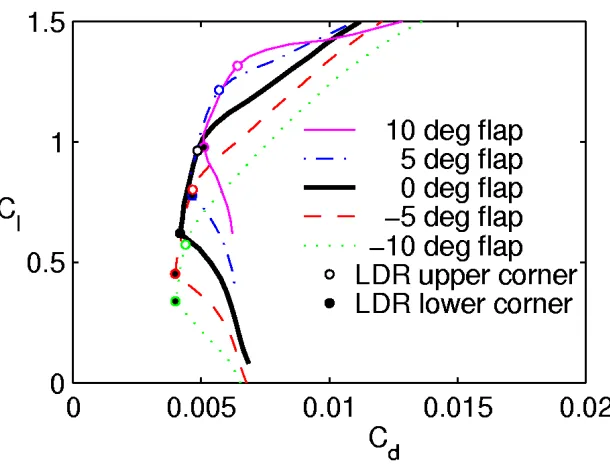
Figure 2.6: SD7037 drag polars with optimal Cl values.
The Spirit 100 uses the SD7037 airfoil [13] designed for efficiency at low Reynolds numbers. As such, its drag polars are affected by phenomena not normally significant at higher Reynolds numbers. Figure 2.6 shows the drag polars for flap angles from−10 to 10 deg at a reduced Reynolds number of 123,000. Asterisks mark the optimalClvalues for each flap from−4 to 10 deg. Note that this optimal value is not theCl at which the airfoil with a certain flap angle has minimum drag. That criteria for optimality would indicate which
angle for a specifiedCl. The aircraft should operate on the Pareto front of all drag polars, which is different than the set of minimum drag positions for each polar. The optimal point for each flap angle is the midpoint of the range ofCl values for which the flap is optimal. For example, a 4 deg flap deflection is optimal forCl values from 0.83 to 0.95. Below 0.83 a 2 deg flap deflection is better, and above 0.95 a 6 deg deflection is better. So the optimal value for a 4 deg deflection is selected as the midpoint of 0.89. This method of determining optimality is better for the purpose of drag minimization.
Figure 2.7: ∆C′
p-Cl curves showing optimalCl values for the SD7037.
For the high Reynolds number NLF airfoils used in previous research, optimal flap angles resulted in ∆C′
range of almost 6 (from −2.1 to 3.7). For the NLF airfoil this range was about 0.1 (from
−0.45 to −0.35). The large spread for the low Reynolds number airfoil means that any constant-∆C′
p controller developed will not be able to optimally minimize drag over all Cl values. However, by careful selection of a constant target ∆C′
p value, the controller can still decrease drag (non-optimally) over some useful range of Cl values. Also, this research is expected to progress toward higher Reynolds number applications where a constant ∆C′
p does minimize drag over reasonable values ofCl. Finally, once the behavior of a constant-∆C′
p controller is understood, a variable-∆Cp′ controller can more easily be developed (if necessary) to minimize drag for low Reynolds number applications.
Figure 2.8: Constant ∆C′
p value of −1.85 for the SD7037. A number of trial ∆C′
Figure 2.9: Drag polars for ∆C′
p target of −1.85 for the SD7037.
of 0.78, the trimClfor the Spirit 100 descending at 0.4 m/s. A ∆Cp′ of−1.85 was selected as the target which the controller would hold constant for purposes of drag reduction. Figure 2.8 shows the data of Fig. 2.7 with asterisks indicating the target ∆C′
p value of−1.85 for each flap value. Figure 2.9 shows the locations of the constant-∆C′
p targets on the drag polars. The target for a 2 deg flap deflection is near optimal around aClof 0.8. Most other targets are not far from optimal, but the drag penalty is fairly large at Cl values above 0.9 or below 0.5. Moving the ∆C′
2.4
Coefficient Determination
There are a number of coefficients that must be determined for use in the controller. ∆C′
p is determined from wing lift, so several coefficients are calculated using it instead of aircraft lift. Wing lift is dependent on angle of attack and flap only, and does not include tail downwash effects. For the purpose of controller development, it is not actual wing lift but incremental wing lift that is important.
∆CLw =CLα,w∆α+CLδf ,w∆δf
=CLα,w∆α+CLα,wτf∆δf
Since the controller must respond to pilot requests from the stick or yoke, it is necessary to know how trim wing lift will be affected for a given elevator deflection (and no flap deflection). Lift and pitching moment equations are manipulated to produce the desired coefficient.
∆CLw =CLα,w∆α
0 = ∆Cm =Cmα∆α+Cmδe∆δe
(dCLw/dδe)Cm=0=
−CLα,wCmδe
Cmα
The following coefficient is presented without explanation since its derivation is similar to that above, except for the use of aircraft lift instead of wing lift.
(dCL/dδe)Cm=0=CLδe −
CLαCmδe
Cmα
One of the controller functions will involve moving the flap and elevator together such that the trim wing lift does not change. It is necessary to know the elevator-to-flap mixing ratio which results in no change to trim wing lift. Lift and pitching moment equations are manipulated to produce the desired coefficient.
0 = ∆CLw =CLα,w∆α+CLδf ,w∆δf
(dδe/dδf)C
Lw=const =
CmαCLδf ,w−CLα,wCmδf
CLα,wCmδe
There are other necessary coefficients that depend on ∆C′
p. These coefficients require analysis of the ∆C′
p data obtained from an airfoil analysis code such as XFOIL [1]. Since the XFOIL results are highly nonlinear at the flap extremities, these coefficients rely on linear fits of data over smaller ranges of flap values. These smaller ranges are selected such that the data in question are fairly linear and include the operating condition about which the aircraft is trimmed.
Figure 2.10: ∆C′
p-δf linear fit for wing lift coefficient of 0.78. It is necessary to know how much flap is required to change ∆C′
of 0.78. Figure 2.8 showed δf-∆Cp′ values over a range of wing lift coefficients. Figure 2.10 shows the result of taking a vertical slice of the data at the trim wingCLof 0.78. The data for flap values below −2 deg or above 6 deg are nonlinear and are rejected. A linear fit of the remaining data produces the following coefficient.
dδf/d∆Cp′
CLw=const= 0.156 rad
Figure 2.11: δf-Cl linear fit for ∆Cp′ =−1.85.
Another value that can be extracted from Fig. 2.8 is the amount of wing lift change due to flap deflection when ∆C′
p is held constant. Figure 2.11 shows the result of taking a horizontal slice of the data at the target ∆C′
deg are nonlinear and are rejected. A linear fit of the remaining data produces the following coefficient.
(dCLw/dδf)∆C′
p=const= 1.98/rad
There are two final coefficients that are needed for the controller. For a given desired change in aircraft CL, how should the flap and elevator be deflected so that ∆Cp′ remains constant? The following equations are used.
∆CL=CLα∆α+CLδe∆δe+CLδf∆δf (2.1a)
0 = ∆Cm =Cmα∆α+Cmδe∆δe+Cmδf∆δf (2.1b)
∆CLw =CLα,w∆α+CLα,wτf∆δf (2.1c)
∆CLw =
h
(dCLw/dδf)∆C′
p=const
i
∆δf (2.1d)
Equation (2.1d) enforces the requirement that as flap changes, the wing lift co-efficient must change such that ∆C′
p is held constant. Combining Eqs. (2.1c) and (2.1d) produces the following.
∆α=γ ∆δf, (2.1e)
whereγ =
(dCLw/dδf)∆C′
p=const
CLα,w
−τf
Substituting Eq. (2.1e) into Eqs. (2.1a) and (2.1b) produces equations for the following coefficients.
(dδf/dCL)∆C′
p=const=
Cmδe
Cmδe
CLαγ+CLδf
−CLδe
Cmαγ+Cmδf
(dδe/dCL)∆C′
p=const=
−Cmαγ+Cmδf
Cmδe
CLαγ+CLδf
−CLδe
Cmαγ+Cmδf
2.5
Controller Functions
The controller has three functions which can be activated independently. The first is gust alleviation. Since the current flap angle and ∆C′
p are available at all times, the instantaneous wing lift can be determined using the data in Fig. 2.8. If the aircraft enters an area of increased updraft, this will increase the angle of attack and thus the lift produced by the wing. As the aircraft flies out of the updraft, the angle of attack and wing lift will decrease. By sending the wing lift through a high-pass filter, lower frequency semi-steady lift values are removed and the resulting signal contains only the higher-frequency gust effects. The gust-alleviation function uses this signal as an error, and thus attempts to minimize the effect of gusts. Figure 2.12 shows a portion of the model for the gust-alleviation function. The error signal is amplified by a proportional gain of 9 to make the flap more effective in reducing the error. This gain value could theoretically reduce the error by 90%, but delays introduced by the flap servo cause the reduction to be less effective. The amplified signal is multiplied by the inverse of−CLδf ,w to determine how much flap is required to offset the wing lift error.
−1 Wing−lift−to−flap derivative −K− Spirit 100 Flap Elevator Wing lift DCPP Proportional gain 9 High−pass filter s s+0.2
Figure 2.12: Partial gust-alleviation function.
The second controller function is ∆C′
p optimization. If the aircraft is operating at a ∆C′
p value other than the target of −1.85, the flap and elevator should be adjusted to bring ∆C′
p back to the target value without changing the wing lift coefficient. Unlike gust alleviation which requires a fast-acting flap, ∆C′
p optimization occurs over a period of several seconds or even tens of seconds. In smooth-air cruising conditions, this delay is insignificant since wing lift changes very slowly. In gusty conditions, ∆C′
p will vary rapidly as wing lift changes. ∆C′
poptimization will slowly adjust the flap and elevator such that the time-averaged value of ∆C′
p is at or near the target value of −1.85. Rapid use of the flap to quickly optimize ∆C′
p would conflict with the gust-alleviation function. For example, an updraft would cause the flap to decrease for gust alleviation, but increase for ∆C′
(steady-state) inputs and ∆C′
p optimization uses a low-pass filter to ignore high-frequency (transient) inputs. Target dcpp −1.85 Spirit 100 Flap Elevator Wing lift DCPP PID Low−pass filter s+0.05 0.05 −1 Flap−to−elevator gain −K− Dcpp−to−flap derivative −K−
Figure 2.13: ∆C′
p-optimization function. Figure 2.13 shows the model for the ∆C′
p-optimization function. The target ∆Cp′ of −1.85 is subtracted from the actual value to determine the error. A low-pass filter with a time constant of 20 seconds removes transients from the error. This filtered error is passed through a PID controller with gains KP = 3.84, KI = 0.192, and KD = 1.28 to improve dynamic response and eliminate steady-state error. The controller output is multiplied by− dδf/d∆Cp′
CLw=const to determine how much flap is needed to correct the ∆C′
p error without changing trim wing lift. The resulting flap command is multiplied by (dδe/dδf)C
Lw=const to determine how much elevator is required to offset the flap deflection
so that trim wing lift does not change. Regardless of what is needed to optimize ∆C′
p, this function always mixes flap and elevator commands such that trim wing lift does not change.
The third controller function is ∆C′
p maintenance. In an aircraft without auto-mated cruise flaps, an elevator deflection causes the aircraft to move from one trim lift coefficient to another. For a given amount of elevator deflection commanded by the pilot, the change in trim lift coefficient can be determined. This lift change will cause steady-state ∆C′
p to change since it is accomplished without any change in flap. If the desired lift change is to be accomplished without changing steady-state ∆C′
p, flap must be deflected as well. This is the purpose of ∆C′
p maintenance. When the pilot provides an elevator input, the controller moves the flap and elevator in a manner such that the desired lift change is provided, but steady-state ∆C′
p does not change (i.e., it is maintained). There are two differences between ∆C′
p maintenance and ∆Cp′ optimization. First, optimization strives to move ∆C′
p to the target value of −1.85 while keeping wing lift constant. Maintenance strives to keep ∆C′
p constant while providing an aircraft lift change requested by the pilot. If the original ∆C′
maintenance attempts to maintain the original value and does not try to move it to −1.85. Second, optimization is concerned with the low-frequency (steadier) ∆C′
p error and thus activates the flap and elevator slowly in response to a time-averaged signal. Maintenance is concerned with instantaneous pilot input from the stick or yoke, and activates the flap and elevator immediately. There is no low-pass filter in the maintenance function to slow flap and elevator motion.
Spirit 100 Flap Elevator Wing lift DCPP Lift−to−flap derivative −K− Lift−to−elevator derivative −K− Elevator−to−lift derivative −K− Pilot 1
Figure 2.14: ∆C′
p-maintenance function. Figure 2.14 shows the model for the ∆C′
p-maintenance function. A pilot request from the stick or yoke is multiplied by (dCL/dδe)Cm=0 to determine the change in trim
aircraft lift that would occur at the requested elevator angle. This lift change is then mul-tiplied by (dδf/dCL)∆C′
p=const and (dδe/dCL)∆Cp′=const to determine the flap and elevator
angles that will provide the requested lift change without changing ∆C′
p.
The issue of interference between the three functions must be addressed. An analysis of frequency responses is useful to determine where there may be problems. The gust-alleviation function uses a high-pass filter with a time constant of 5, so its frequency domain of interest is primarily 0.2 rad/s and above. The ∆C′
p-optimization function uses a low-pass filter with a time constant of 20, so its domain is primarily 0.05 rad/s and below. These two functions are unlikely to interfere with each other because their frequency domains do not intersect. The ∆C′
p-maintenance function does not filter its input, so all frequencies are in its domain. Its behavior must be examined with respect to each of the other functions.
The ∆C′
p-optimization function attempts to drive ∆Cp′ to the target value of−1.85. After it has been activated for some time, the value will either be very close to −1.85 (in smooth conditions) or varying around a mean close to −1.85 (in gusty conditions). If the pilot then requests a change in lift using the stick or yoke, the ∆C′
∆C′
p of −1.85. Since both the optimization and maintenance functions are striving for the same ∆C′
p (−1.85), they complement each other and there is no interference.
The gust-alleviation function uses rapid flap motions to minimize deviations from the current wing lift coefficient. If the pilot requests a change in lift, the ∆C′
p-maintenance function will attempt to provide this change, but the gust-alleviation function will quickly activate the flaps to prevent any change. These two functions will interfere with each other. This undesirable behavior would occur even if the ∆C′
p-maintenance function were deactivated and the pilot directly controlled the elevator. Any attempt to change lift would be opposed by the gust-alleviation function.
−1 Wing−lift−to−flap derivative −K− Spirit 100 Flap Elevator Wing lift DCPP Proportional gain 9 High−pass filter s s+0.2 Elevator−to−wing−lift derivative −K− Pilot 1
Figure 2.15: Gust-alleviation function.
For this reason the gust-alleviation function must be modified slightly to take into account lift changes requested by the pilot. Figure 2.15 shows the complete model for the gust-alleviation function. Pilot input from the stick or yoke is multiplied by (dCLw/dδe)Cm=0
to determine the change in wing lift at the new trim condition for the requested elevator angle. This desired lift is subtracted from the actual wing lift to create a lift coefficient error which is then sent to the high-pass filter. From this point on the operation of the function is identical to that previously described, because subtracting out the pilot-commanded change in lift merely alters the reference point of the signal entering the high-pass filter.
2.6
Controller Performance
discretely at approximately 220 Hz. Figure 2.16 shows the first 60 seconds of the vertical gust profile resulting from the model. The noise power was selected such that the size of an average gust is about 0.08 m/s, or about 1% of aircraft speed. There is no horizontal (longitudinal or lateral) gust component.
Figure 2.16: Gust profile.
Figure 2.17 shows a 120-second simulation in which all controller functions are initially inactive, and the gust-alleviation function is activated at 60 seconds. Gust allevia-tion is effective in minimizing disturbances in both aircraft lift and the G force felt at the aircraft center of gravity. Peak values for both parameters are reduced by about 65%. The trade-off for this improvement is an increase in deviations about the mean ∆C′
opposite to the direction required to restore the previous ∆C′
p, so this increase in deviations is expected.
The gust-alleviation function requires rapid movement of the flap and precise knowledge of the instantaneous value of ∆C′
p. In the simulation, simplifying assumptions are made for the flap servo and ∆C′
p determination. The flap servo is modeled as a continuous-time component (second-order filter), and ∆C′
p is determined using instantaneous coefficient of lift provided by the AeroSim blockset. In a flight test environment, R/C servo signals are typically generated 50 times per second, and this limits how quickly the servo can react. The measured value of ∆C′
pis also likely to be affected by unsteady aerodynamics and lag in the sensing system. Therefore, the gust-alleviation function may be difficult to implement and evaluate in a flight test environment.
Figure 2.18 shows a simulation in which all controller functions are again initially inactive and the ∆C′
p-optimization function is activated at 60 seconds. Over a period of about 10 seconds, the flap and elevator activate to drive ∆C′
p from its starting value of about −2.04 toward the target value of −1.85. This is done without significant effects to the other aircraft parameters. This indicates that a slow-acting ∆C′
p-optimization function could be added to an aircraft without causing undesirable changes to its dynamic response. Figure 2.19 shows two responses to a request from the pilot for a−1 deg elevator change. In the uncontrolled case, the request (at 10 seconds) is passed directly to the elevator and a classic phugoid response is observed. ∆C′
pchanges (as expected) from−2.04 and oscillates around a mean of about−2.27. At 60 seconds, the ∆C′
p-maintenance function is activated, and the next −1 deg request (at 70 seconds) is converted to a −0.202 deg elevator deflection and a +2.65 deg flap deflection. This combination results in the same phugoid response as the uncontrolled case, but the ∆C′
p oscillation is now about the original value and thus the steady-state ∆C′
p has not changed much. Since parameters other than ∆C′
p are virtually identical between the two cases, a fast-acting ∆Cp′-maintenance function could also be added to an aircraft without undesirable dynamic response changes.
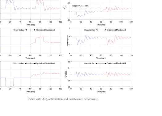
Figure 2.20 is similar to Fig. 2.19 except that both the ∆C′
p-optimization and maintenance functions are activated at 60 seconds. Within about 10 seconds, ∆C′
p has moved from the initial value of −2.04 toward the target value of −1.85. When the pilot input is received at 70 seconds, ∆C′
p oscillates about the current (and target) value of
of the uncontrolled (elevator only) aircraft. This indicates that a function implementing both slow-acting ∆C′
p optimization and fast-acting ∆Cp′ maintenance could be added to an aircraft without adverse effects.
For the final simulation, all three controller functions (gust alleviation, ∆C′
p op-timization, and ∆C′
p maintenance) are activated at 60 seconds. The inputs include the previously-discussed gust profile and pilot requests from the stick or yoke. Figure 2.21 shows that gust alleviation is effective at reducing lift-coefficient perturbations (including phugoid oscillations) by about 65%. Reduction of G-force perturbations averages about 40%, but is dependent on pilot input. Perturbations immediately after a pilot input (at 70 and 85 seconds) are actually worse with the control functions activated than with the func-tions inactive (at 10 and 25 seconds). However, these increased G-force perturbafunc-tions occur only in response to aircraft stick or yoke movement, so changes in G force will be expected by the pilot. After the aircraft is able to settle into a steady-state condition (except for gusts), the controlled system has lower G-force perturbations than the uncontrolled system. Airspeed perturbations are initially similar for both systems, but damp out quicker with the controller functions activated.
The simulations performed illustrate the effectiveness of using a three-function con-troller based on ∆C′
p data. Positive results were observed when the functions were tested separately, as well as when all functions were activated simultaneously. Gust alleviation was successful in reducing aircraft lift and G-force perturbations in almost all instances. It also had the added effect of reducing phugoid oscillations. ∆C′
poptimization was successful in maintaining a mean target ∆C′
p value, which reduced drag for the low Reynolds number SD7037 airfoil and should minimize drag for higher Reynolds number NLF airfoils. ∆C′
p maintenance was successful in preventing large ∆C′
p changes due to pilot input. Although these changes would eventually be eliminated by the ∆C′
p-optimization function, mainte-nance prevents them from occurring and thus allows mean ∆C′
Figure 2.18: ∆C′
Figure 2.19: ∆C′
Figure 2.20: ∆C′
Chapter 3
Controller Hardware/Software
3.1
Overview
This chapter presents the details of the hardware and software which were used to implement the flight-ready automated cruise flap controller. It discusses how controller functionality is broken down into simple tasks that can be executed by one of five separate modules. It also explains the communication scheme that was developed to allow data to be passed from one module to another.
3.2
General Information
The controller was implemented using 8-bit PIC microcontrollers from Microchip Technology, Inc. Custom assembly language software for the microcontrollers was developed on a Linux workstation using the open-source gputils [14] package. Assembled code was downloaded to the microcontrollers using a Microchip PICkitTMUSB Programmer and the usb pickit[15] program. The source code [16] for the software implementing the controller is available for download.
The controller was developed in an incremental fashion, and flight tests were per-formed to ensure that each newly developed section of code operated correctly. For the first flight test day, July 12, 2008, only the code to measure ∆C′
p was complete. Results from this test day indicated the need to modify the manner in which ∆C′
p values were recorded. This change to the software was made, and the new ∆C′
implemen-tation of the ∆C′
p-maintenance function, and this was tested on August 6, 2008. The final step was development of the ∆C′
p-optimization function. On the fourth test day of August 15, 2008, the controller was tested with both the ∆C′
p-maintenance and ∆Cp′-optimization functions operational. As a result of the incremental development and testing cycle, there were many different versions of the software throughout the process. The versions of the software and hardware described in this chapter are the final versions that were used for flight tests on August 15, 2008.
The controller is composed of five different modules. Each module is comprised of a single microcontroller and the software necessary to carry out the task of the module. The five modules are:
• DCPP reader: Calculates raw ∆C′
p and filtered ∆Cp′ error using analog voltages output by the pressure transducers.
• Servo reader: Measures the pulse widths of the servo signals from the R/C receiver
for the flap, elevator, aileron, and landing gear channels.
• Servo writer: Converts desired servo positions into pulses of appropriate widths that
are sent to the flap, elevator, left aileron, and right aileron servos.
• Servo calculator: Calculates desired servo positions using data obtained from the
reader modules and sends these positions to the servo writer.
• Fail-safe switch: Monitors the landing gear signal from the R/C receiver to
deter-mine if the controller is enabled, and routes either receiver or controller signals to the servos, as appropriate.
3.3
Communications Scheme
To allow data to be passed from one module to another, a communications scheme was developed. All modules are connected to a trigger line and a data line. The servo calculator is able to write to the trigger line, and all other modules are only able to read from the line. Reader and writer modules listen for a triggering pulse which indicates that they should perform some action or write their information to the data line. Thus, the servo calculator acts as the “pacemaker” that drives the process which eventually moves the servos.
There are three types of messages, and each has a distinct message ID. Each message commands a reader or writer module to perform some action.
• Message ID 0: Causes the DCPP reader to write raw ∆C′
p and filtered ∆Cp′ error values on the data line.
• Message ID 1: Causes the servo reader to write R/C receiver flap, elevator, and
aileron servo positions on the data line, as well as a flag indicating whether the pilot has enabled the controller.
• Message ID 2: Causes the servo writer to listen for controller flap, elevator, and
aileron positions on the data line and convert them to pulses of appropriate widths which are sent to the servos.
When a message with a specific ID needs to be generated, the servo calculator writes a pulse of the appropriate width to the trigger line. The width of the pulse is (50 + 10n) microseconds, where n is the ID number of the message. The trigger pulse for message ID 1, for example, is 60µsec long. Other modules listen on the trigger line for the beginning of a pulse, and then time the pulse to determine its width, and therefore its ID. If the ID is one to which they do not respond, they ignore the request and listen for the next trigger pulse. In general, modules use interrupts to be notified of the beginning of a trigger pulse. This allows them to focus on any continuously-running tasks they have, since they will be interrupted to handle a trigger pulse whenever one begins.
input is placed in high-impedance mode, meaning the microcontroller does not drive the pin voltage at all and it is free to take whatever voltage is placed on it by outside circuitry. In most common microcontroller applications, each pin is configured as input or output by the initialization code and is never again changed. It is not possible to follow that practice in this communication scheme.
There are three modules that write to the data line: DCPP reader, servo reader, and servo calculator. Each module must therefore have one pin connected to the data line. Assume that each of these pins has been configured for output in the initialization code, so each of them are driving a voltage on the data line. At start-up, the output pins are initialized to 0 volts, so all three modules are driving the data line to that value and there is no problem yet. When a pulse corresponding to message ID 0 is written to the trigger line, the DCPP reader will begin writing data to the data line. The first bit to be written is a start bit, which is a logical 1, so the DCPP reader drives the data line to 5 volts. At the same time, the other two modules are driving the same line to 0 volts, and a short circuit occurs. This results in a huge current through the data line, and voltages in all microcontrollers drop to the point that they cease operation and reset themselves.
To prevent this from occurring, the data lines are configured as inputs in the initialization phase, and normally remain so. Immediately before they write data on the data line, they are reconfigured as outputs. After the data are written, they are changed back to inputs. In theory, this means that only one microcontroller should have its data line pin configured as an output at any given time, and this prevents the short circuit that will reset the microcontrollers.