University of Windsor University of Windsor
Scholarship at UWindsor
Scholarship at UWindsor
Electronic Theses and Dissertations Theses, Dissertations, and Major Papers
10-19-2015
Predicting Composite Material Performance for LFT-D Using
Predicting Composite Material Performance for LFT-D Using
Processing Parameters
Processing Parameters
Xu Zhang
University of Windsor
Follow this and additional works at: https://scholar.uwindsor.ca/etd
Recommended Citation Recommended Citation
Zhang, Xu, "Predicting Composite Material Performance for LFT-D Using Processing Parameters" (2015). Electronic Theses and Dissertations. 5480.
https://scholar.uwindsor.ca/etd/5480
This online database contains the full-text of PhD dissertations and Masters’ theses of University of Windsor students from 1954 forward. These documents are made available for personal study and research purposes only, in accordance with the Canadian Copyright Act and the Creative Commons license—CC BY-NC-ND (Attribution, Non-Commercial, No Derivative Works). Under this license, works must always be attributed to the copyright holder (original author), cannot be used for any commercial purposes, and may not be altered. Any other use would require the permission of the copyright holder. Students may inquire about withdrawing their dissertation and/or thesis from this database. For additional inquiries, please contact the repository administrator via email
Predicting Composite Material Performance for LFT-D Using
Processing Parameters
By
Xu Zhang
A Thesis
Submitted to the Faculty of Graduate Studies
through the Department of Mechanical, Automotive, and Materials Engineering in Partial Fulfillment of the Requirements for
the Degree of Master of Applied Science at the University of Windsor
Windsor, Ontario, Canada
2015
Predicting Composite Material Performance for LFT-D Using Processing Parameters
by
Xu Zhang
APPROVED BY:
______________________________________________ Dr. Edrisy
Department of Mechanical, Automotive, and Materials Engineering
______________________________________________ Dr. Minaker
Department of Mechanical, Automotive, and Materials Engineering
______________________________________________ Dr. Johrendt, Advisor
Department of Mechanical, Automotive, and Materials Engineering
DECLARATION OF ORIGINALITY
I hereby certify that I am the sole author of this thesis and that no part of this thesis
has been published or submitted for publication.
I certify that, to the best of my knowledge, my thesis does not infringe upon anyone’s
copyright nor violate any proprietary rights and that any ideas, techniques, quotations, or
any other material from the work of other people included in my thesis, published or
otherwise, are fully acknowledged in accordance with the standard referencing practices.
Furthermore, to the extent that I have included copyrighted material that surpasses the
bounds of fair dealing within the meaning of the Canada Copyright Act, I certify that I
have obtained a written permission from the copyright owner(s) to include such material(s)
in my thesis and have included copies of such copyright clearances to my appendix.
I declare that this is a true copy of my thesis, including any final revisions, as
approved by my thesis committee and the Graduate Studies office, and that this thesis has
ABSTRACT
Carbon fiber-reinforced composite material properties can be directly related to the
manufacturing process. No generally accepted model or system exists that can model the
relationship between manufacturing process parameters and composite material properties.
The purpose of this research is to develop an artificial neural network model to predict the
manufacturing process parameters’ influence on the properties of carbon fiber-reinforced
composite material. Different types of artificial neural networks are compared in current
research in order to obtain the best prediction results. In this research, the calculated
sensitivities from the trained neural network are used to find the effect of processing on
material properties. Finally, a complete artificial neural network model for predicting
To my loving parents, Lirong and Junfeng,
And my loving wife, Rui,
ACKNOWLEDGEMENTS
There are a number of people without whom this journey would have not been
possible. I am forever indebted to them. I would also like to thank the International
Composites Research Centre at Western University and Fraunhofer Project Center at
London, Ontario for their funding support and internship opportunity.
Foremost, I would like to express my deepest gratitude and appreciation for my
supervisor, Dr. Jennifer Johrendt, for her patience, knowledge, motivation, technical
guidance, and kindness. It is extremely fortunate for me as one of her Master students and
I am very appreciative of her for believing in me and giving me lots of confidence. I
would also like to thank my committee members, Dr. B. Minaker and Dr. A. Edrisy, for
their support and comments. Thanks to the help and advice from PhD candidate Matthew
Bondy and PhD candidate Zhe (Tom) Ma. They gave me lots of guidance on technique
and gave me confidence to finish this research.
I would also like to thank PhD candidate Ying Fan in Western University who
provided the test data applied in this research. Thanks to Kaptur Louis at FPC who
patiently provided me all the LFT-D manufacturing processing data and technical
guidance on the machine.
There are some very special people that I would like to acknowledge and to whom I
express my sincerest gratitude. I would like to thank my parents, Lirong and Junfeng, for
believing in me and their unlimited supporting for my twenty-year studying period. I
CONTENT
DECLARATION OF ORIGINALITY ... iii
ABSTRACT ... iv
ACKNOWLEDGEMENTS ... vi
LIST OF TABLES ... x
LIST OF FIGURES ... xi
LIST OF ABBREVIATIONS/NOMENCLATURE ... xiii
LIST OF SYMBOLS ... xiv
CHAPTER 1 INTRODUCTION ... 1
CHAPTER 2 THEORY ... 4
2.1 Composite Material ... 4
2.1.1 Composite Material Structures ... 5
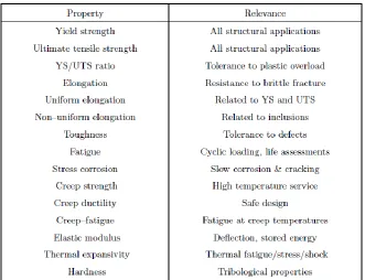
2.1.2 Constituent Properties ... 7
2.2 Carbon Fiber Composite Materials ... 16
2.2.1 Fiber Composite Materials Classifications ... 16
2.2.2 Continuous Carbon Fiber Polymer-matrix Composite Properties ... 17
2.3 Composite Material Process Methods ... 18
2.3.1 Processing of Thermoset Matrix Composites ... 18
2.3.2 Processing of Thermoplastic Matrix Composites ... 20
2.3.3 Introduction to RTM, Injection Molding, SMC, and LFT-D-ILC ... 22
2.3.4 LFT-D Processes ... 26
2.4 Introduction to Neural Networks ... 29
2.4.1 Introduction to Neural Networks ... 29
2.4.2 Training of Neural Networks ... 34
2.4.3 Learning of Neural Networks... 39
2.4.4 Training Methods Summary ... 43
2.5 Chapter Summary ... 45
CHAPTER 3 LITERATURE REVIEW ... 46
3.1.1 M. Al-Assadi et al. ... 49
3.1.2 Hany El Kadi et al. ... 50
3.1.3 J.A. Lee et al. ... 51
3.1.4 Yousef Al-Assaf and Hany El Kadi ... 53
3.1.5 Others ... 54
3.2 Predicting Composite Material Strength Using ANNs ... 54
3.2.1 Mohammed A. Mashrei et al. ... 54
3.2.2 Z. Zhang et al. ... 56
3.3 Predicting Other Properties of Composite Materials with ANNs ... 58
3.4 Predicting Material Performance using Neural Network Sensitivity ... 60
CHAPTER 4 COLLECTION AND SELECTION OF DATA ... 62
4.1 Data Resource ... 62
4.2 LFT-D Processing Parameters ... 63
4.2.1 Mean Data ... 63
4.2.2 Data Standard Deviation ... 64
4.2.3 Data Normalization ... 65
4.2.4 Reversing the Normalization... 66
4.3 Material Test Data ... 66
4.3.1 Young’s Modulus and Tensile Strength ... 68
4.3.2 Test Data Organization ... 68
CHAPTER 5 NEURAL NETWORK PREDICTION ... 70
5.1 Function Selection ... 70
5.2 Training Method Selection ... 71
5.2.1 Network Types ... 72
5.2.2 Adaption Learning Functions ... 73
5.2.3 Comparison of Network Types ... 75
5.2.4 Section Summary ... 77
5.3 Hidden Layer Configuration ... 78
5.3.1 Number of Hidden Neurons ... 78
5.3.2 Number of Hidden Layers ... 80
5.4 Artificial Neural Network Training ... 85
5.4.1 Network Training using Mean Value of Processing Parameters ... 86
5.4.2 Network Training using Standard Deviation of Processing Parameters ... 87
5.4.3 ANN Development to Predict CFRP Properties Using LFT-D Processing Parameters 87 5.5 Sensitivity of Network Outputs to Network Inputs ... 91
5.5.1 Sensitivity Analysis ... 92
5.5.2 Neural Network Optimization ... 101
CHAPTER 6 RESULT ANALYSIS ... 105
CHAPTER 7 CONCLUSIONS AND RECOMMENDATIONS ... 106
7.1 Conclusions ... 106
7.2 Recommendations ... 108
REFERENCE ... 109
APPENDIX ... 111
Appendix A ... 111
Appendix B ... 118
Appendix C ... 122
Appendix D ... 126
LIST OF TABLES
TABLE 2.1.1CLASSIFICATION OF COMPOSITE MATERIALS ... 6
TABLE 2.1.2GLASS FIBER COMPOSITIONS AND PROPERTIES... 9
TABLE 2.1.3TYPICAL PROPERTIES OF E-GLASS FIBERS ... 10
TABLE 2.1.4TYPICAL STRUCTURAL MATRIX RESINS ... 15
TABLE 3.1MECHANICAL PROPERTIES ... 46
TABLE 3.2RMSE FUNCTION OF THE TYPE OF ARCHITECTURE AND TRAINING FUNCTION .. 50
TABLE 3.3COMPARISON OF NMSE AND R ... 51
TABLE 3.4MEAN ABSOLUTE ERROR BETWEEN EXPERIMENTAL AND PREDICTIONS RESULTS 53 TABLE 3.5COMPARISON OF BOND STRENGTH PREDICTION ... 55
TABLE 3.6COMPARISON OF CORRELATION COEFFICIENT,R ... 55
TABLE 4.1STANDARD DEVIATION AND MEAN OF INPUT DATA ... 69
TABLE 5.1THE ERROR OF DIFFERENT NETWORKS WITH DIFFERENT TRANSFER FUNCTIONS . 70 TABLE 5.2PERFORMANCE OF EACH LEARNING FUNCTION ... 74
TABLE 5.3ALTERNATIVE OPTIONS OF THE NETWORK TYPES ... 75
TABLE 5.4PERFORMANCE (MSE) OF DIFFERENT HIDDEN NEURONS ... 83
TABLE 5.5NETWORK TRAINING PARAMETERS ... 86
TABLE 5.6PERFORMANCE OF THE MEAN VALUE DATA TRAINED RESULT ... 87
TABLE 5.7PERFORMANCE OF STANDARD DEVIATION DATA RESULT ... 87
TABLE 5.8ARTIFICIAL NEURAL NETWORK TRAINING PARAMETERS... 88
TABLE 5.9THE MEAN VALUE OF THE SUMMED ABSOLUTE SENSITIVITIES ... 94
TABLE 5.10BEST VALIDATION PERFORMANCE OF DIFFERENT TRAINING FOR NETWORK ... 98
LIST OF FIGURES
FIGURE 2.1.1TYPES OF FIBER-REINFORCED COMPOSITES ... 6
FIGURE 2.1.2SCHEMATIC OF GLASS FIBER MANUFACTURE ... 10
FIGURE 2.1.3(A)STRUCTURE OF GRAPHITIC LAYER.THE LAYERS ARE SHOWN NOT IN CONTACT FOR VISUAL EASE.(B)THE HEXAGONAL LATTICE STRUCTURE OF GRAPHITE . 11 FIGURE 2.1.4SCHEMATIC REPRESENTATION OF THE STRUCTURE OF CARBON FIBERS ... 12
FIGURE 2.1.5MATERIAL PROPERTIES OF CFRPS GOVERNING THE MACHINE ABILITY OF CFRPS ... 13
FIGURE 2.1.6POSSIBLE ARRANGEMENTS OF POLYMER MOLECULES:(A)AMORPHOUS,(B) SEMI-CRYSTALLINE ... 14
FIGURE 2.1.7DIFFERENT TYPES OF COPOLYMERS ... 15
FIGURE 2.31(A) IN HAND LAYUP, FIBERS ARE LAID ONTO A MOLD BY HAND AND THE RESIN IS SPRAYED OR BRUSHED ON (B) IN SPRAY-UP, RESIN AND FIBERS (CHOPPED) ARE SPRAYED TOGETHER ONTO THE MOLD SURFACE ... 19
FIGURE 2.32(A) SCHEMATIC OF FILAMENT WINDING PROCESS.(B)SCHEMATIC OF A FILAMENT WOUND PRESSURE VESSEL WITH A LINER; HELICAL AND HOOP WINDING ARE SHOWN ... 19
FIGURE 2.33SCHEMATIC OF THE PULTRUSION PROCESS ... 20
FIGURE 2.34VARIATION OF SOME MECHANICAL PROPERTIES OF A COMPOSITE AS A FUNCTION OF FIBER LENGTH ... 24
FIGURE 2.35EXTRUSION/COMPRESSION MOLDING PROCESS FOR MAKING LONG FIBER REINFORCED THERMOPLASTIC (LFT) COMPOSITES. ... 25
FIGURE 2.36PROCESS SCHEME OF LFT-D LINE ... 27
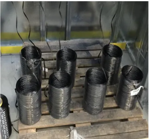
FIGURE 2.37 CARBON FIBER IN ROVINGS PREPARED FOR LFT-D FEEDING ... 27
FIGURE 2.38CHARGE PRODUCED BY LFT-D PREPARED FOR PRESS ... 28
FIGURE 2.39TEST PANELS PRODUCED BY LFT-D PROCESS ... 28
FIGURE 2.41A2-5-1 BACKPROPAGATION FEED-FORWARD NEURAL NETWORK CONFIGURATION ... 30
FIGURE 2.42SOME NONLINEAR NEURON TRANSFER FUNCTIONS:(A)LOGISTIC,(B) HYPERBOLIC-TANGENT,(C)GAUSSIAN,(D)GAUSSIAN COMPLEMENT,(E)SINE FUNCTION ... 31
FIGURE 2.43SIMPLE 1-1-1 NEURON NETWORK CONFIGURATION ... 35
FIGURE 2.44 M-N-L LOGSIG PURELIN NEURAL NETWORK CONFIGURATION ... 37
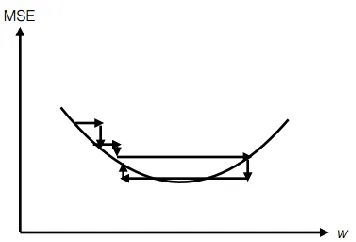
FIGURE 2.45OPTIMAL LEARNING RATE FOR EFFICIENT ERROR MINIMIZATION ... 40
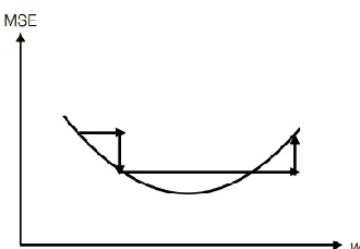
FIGURE 2.46EFFECT OF A HIGH RATE ON LEARNING ... 40
FIGURE 2.47EFFECT OF TOO HIGH A LEARNING RATE ON LEARNING ... 41
FIGURE 3.1OUTLINE OF THE NETWORK ... 48
FIGURE 3.2A TWO-LAYER RECURRENT ELMAN NEURAL NETWORK ARCHITECTURE ... 49
FIGURE 3.3RESULTS OF TRIALS TO ESTABLISH THE OPTIMUM ARCHITECTURE ... 52
FIGURE 3.4SCHEMATIC PRESENTATION OF HOW TO DESIGN THE COMPOSITION OF WEAR RESISTANT POLYMER COMPOSITES ... 56
FIGURE 3.5INPUT DATA,OUTPUT DATA AND SCHEMATIC CONSTRUCTION OF AN ANN ... 57
FIGURE 3.6THE FLOW CHART OF BPNN TRAINING AND OPTIMIZATION ... 59
FIGURE 4.1LFT-D PROCESSING PARAMETERS CLASSIFICATION ... 64
FIGURE 4.3CARBON FIBER-REINFORCED THERMOPLASTIC PANELS PRODUCED BY LFT-D . 67
FIGURE 5.1HIDDEN NEURONS AND OUTPUT NEURONS SCHEMES ... 71
FIGURE 5.2 MATLAB NEURAL NETWORK WORK SHOP WINDOW ... 72
FIGURE 5.3CONFIGURATION OF A 2-HIDDEN-LAYER CASCADE-FORWARD NETWORK ... 73
FIGURE 5.4THE CONFIGURATION OF A 2-HIDDEN-LAYER ELMAN NETWORK ... 73
FIGURE 5.5TRAINING PARAMETERS ... 79
FIGURE 5.6BEST RESULTS COMPARE WITH EXPECTED CURVE ... 79
FIGURE 5.7TRAINING PARAMETERS FOR DIFFERENT NUMBER OF HIDDEN LAYERS ... 80
FIGURE 5.8THE ARCHITECTURES OF TWO ANNS ... 81
FIGURE 5.9 (A)MSE OF 1-HIDDEN-LAYER TRAINING (B)MSE OF 2-HIDDEN-LAYER TRAINING ... 82
FIGURE 5.10PERFORMANCE (MSE) OF DIFFERENT HIDDEN NEURONS IN A ONE HIDDEN LAYER LOGSIG-PURELIN NEURAL NETWORK ... 84
FIGURE 5.11PERFORMANCE OF NEURAL NETWORK WITH DIFFERENT NUMBER OF HIDDEN NEURONS ... 85
FIGURE 5.12NEURAL NETWORK CONFIGURATION FOR TRAINING ... 86
FIGURE 5.13TRAINING STATUS OF NEURAL NETWORK APPLIED FOR CURRENT RESEARCH .. 89
FIGURE 5.14VALIDATION, TRAINING, AND TEST MSE ... 90
FIGURE 5.15REGRESSION OF NETWORK TRAINING RESULTS: REGRESSION OF ORIGINAL DATA ... 91
FIGURE 5.16COMMON DESCRIPTIONS OF NEURONS FOR REGULAR NEURAL NETWORK ... 92
FIGURE 5.17(A) TO (D) THE MEAN OF THE SUMMED ABSOLUTE SENSITIVITIES FOR OUTPUTS TO INPUTS FROM OUTPUT Z1 TO Z4 ... 96
LIST OF ABBREVIATIONS/NOMENCLATURE
ANNs Artificial Neural Networks BPNN Backpropagation Neural Network CC Carbon-Carbon Composites
CFB Cascade-Forward Backpropagation CFRP Carbon Fiber-Reinforced Plastic CMC Ceramic Matrix Composites D-SMC Direct Sheet Molding Compound EB Elman Propagation
FFB Feed-Forward Backpropagation FPC Fraunhofer Project Centre
FRP Fiber-Reinforced Polymer/Plastic GFRP Glass Fiber-Reinforced Plastic HC Hybrid Composites
LFT Long Fiber Thermoplastic Compression Molding LFT-D Direct Long Fiber Thermoplastic Compression Molding LM Levenberg Marquardt Training Algorithm for ANN MLP Multi-Layer Perceptron
LIST OF SYMBOLS
𝑥𝑖 ith neural network input
𝑤𝑖𝑗 neural network weight and bias
from the ith input to the jth hidden neuron
𝑏𝑗 neural network weight and bias
from the jth hidden neuron to the network output
µ𝑖 weighted sum of inputs in to the ith hidden neuron
ѵ𝑖 weighted sum of hidden-neuron output from the ith hidden neuron
𝑛 number of input neurons
𝑙 number of hidden neurons
𝑚 number of output neurons
𝑦𝑗 calculated result of weighted sum of inputs in neural network
𝑧𝑘 calculated result of weighted sum of hidden-neuron output
𝐸 mean square error
𝜀 neural network learning rate
𝑑𝑔 total gradient of network
𝑔 neural network training epoch number
∆𝑤 hidden weights and bias update
CHAPTER 1 INTRODUCTION
Composite materials are widely used in mechanical engineering to satisfy specific
industrial requirements. Composites are a combination of two or more materials with
different properties, whose combination produces a new material with beneficial
properties for specific application. In the automotive and aviation fields, lighter, stronger
and lower cost materials are always required, making composites an obvious choice.
One of the typical engineered composite materials used by these industries is reinforced
plastic. Currently, increased research is being done in the automotive industry regarding
the use of Fiber-Reinforced Plastics (FRP) in automotive applications in order to improve
fuel economy by reducing the vehicle weight.
Many automotive companies have already applied lightweight materials to their
vehicle designs like carbon fiber or glass fiber reinforced plastics, for example on
Renault’s new concept light-weight design car which only consumes 1 litre per 100km
(Group 2014). In luxury cars and race cars, carbon fiber composites are generally used in
inner trim and car body applications. Currently, additional applications are being
investigated such as trunk lids, exhaust pipes, and the engine head.
Western University, in London, Ontario, Canada, and the Fraunhofer Institute of
Chemical Technology (ICT) in Pfinztal, Germany, have launched long-term research
collaboration on composite technologies for weight reduction. The University of Windsor,
McMaster University, and the University of Toronto are Canadian members of this project
as well through their membership in the International Composite Research Centre (ICRC).
This comprehensive initiative, Fraunhofer Project Centre (FPC) for composite materials
at Western, is working on design and development of composite technologies to achieve
required material properties with industrial partners in the automotive industry.
One of the key research missions at FPC is to produce and analyze lightweight
composite materials. FPC has four technologically advanced machine lines that produce
manufactures and academic research, FPC conducted trials to produce composite material
panels with continuous and chopped glass fibers or carbon fibers in different various
configurations.
In the automotive industry, applications of FRP can be classified into chassis, body,
and engine components. For chassis components, many researchers have used
fiber-reinforced composite in the manufacture of leaf spring and drive shafts. The high
temperature requirement of the matrix (i.e. resin) component is a big challenge for
composite engine components. Due to the complex structure and complicated process of
manufacturing FRP materials, it cannot be analyzed with the same methods as singular
component material. Therefore, there is a need for a simplified model that can accurately
relate manufacturing properties and the performance of FRPs.
Artificial Neural Networks (ANNs) are such tool that can be used to predict
mechanical properties of composite materials in this way. This black-box model has many
advantages like global optimal searching and quick convergence speed (J. Xu 2007).
Additionally, ANNs can be applied not only in the study of mechanical properties but
wherever the complexity of a problem is overwhelming from a fundamental perspective
and where over-simplification is unacceptable in the face of reduced accuracy (H. K.
Bhadeshia 1999).
One goal of the current research is to use ANNs to determine the relationship
between FRP performance and the manufacturing process parameters. Thus, there are
three main topics relevant to the current research: composite materials, composite
materials manufacturing processes, and neural network modeling.
This thesis focused on analyzing continuous carbon fiber-reinforced thermoplastic
composite material (CFRP) which is produced by the LFT-D machine line (Direct Long
Thermoplastic Molding) at FPC. As such, ANNs were developed relating the LFT-D
processing parameters (model inputs) to mechanical properties of the material (model
ICRC researchers at the University of Western Ontario.
In this thesis, Chapter 2 introduces the basic theories of the research, including
composite material classification and properties with respect to the geometry. Additionally,
some traditional methods and advanced methods of composite materials manufacturing
are introduced as well as a basic introduction to ANNs.
A review of relevant literature is included in Chapter 3, providing background concerning
composite material analysis and neural network prediction. Specifically, some literature
highlighting the use of ANNs in composite material modeling provide examples ANN
applications in this field.
In Chapter 4, details of how to design and develop neural networks will be given. The
CHAPTER 2 THEORY
The aim of this research is to model the relationship between the material processing
parameters and the material performance. As such, it is necessary to develop an
understanding of the composite materials as well as the material manufacturing process.
Additionally, a foundation in neural networks is also necessary. In this chapter, there are
three sections: composite materials, composite material processing method, and neural
networks.
2.1 Composite Material
In fact, composite materials have been used since ancient times to enhance the
material properties. For instance, the civil engineers placed steel rebar in cement and
aggregate to make a well-known composite material, i.e., reinforced concrete in 20th century (Jack R. Vinson and Robert L. Sierakowski, 2008). This research is focused on
the advanced composite materials that are widely used in today’s industrial applications.
To provide a more specific description of simple composite materials, there are two
main categories of composite material components: the matrix and reinforcement
(Chawla 2012). With a specific proportion of each component, the reinforcement is
surrounded and supported by the matrix. The matrix performance is improved by
mechanical and physical properties of the reinforcement. Additionally, composite
materials are classified based on their material properties, another important aspect to
study (Jack R. Vinson and Robert L. Sierakowski, 2008).
The properties of composite materials are dependent on the material components, the
proportion and distribution of the components, the structure of the materials’
crystallography, as well as the manufacturing process of the material. As this research is
focused on the performance of one kind of composite material, the many factors’
influence will be described specifically in a later section (Chawla 2012).
specific requirements by varying the amount and layout of composite components. One
key advantage of composite materials used for in automotive applications is lightweight
structure (Jack R. Vinson and Robert L. Sierakowski, 2008).
A common type composite material is fiber reinforced polymer (FRP) that is the
focus of this research. The properties of FRPs can be highly influenced by the material
characteristics of the fiber rather than that of the matrix. The arrangement, the shape, the
specification, and the construction of the fibers are the primary factors that influence the
performance of the FRP. In the automotive industry, there are two types of widely used
FRPs: carbon fiber-reinforced polymer (CFRP) and glass fiber-reinforced polymer
(GFRP).
After composite material structures and constituents are explained in general, CFRP
will be described as the focus in this research.
2.1.1 Composite Material Structures
Composite materials are classified according to their structure. The three levels of
structure for consideration with respect to the constituent elements of advanced composite
materials are (Jack R. Vinson and Robert L. Sierakowski, 2008):
(1) Basic/Elemental: single molecules, crystal cells;
(2) Micro structural: crystals, phases, compounds;
(3) Marco structural: matrices, particles, fibers.
In general, the macrostructure level of composite material is the focus of main
research topics today. In order to obtain a clear understanding of composite materials, it is
important to review classifications of composite materials as described by the forms of
Table 2.1. 1 Classification of composite materials (Chawla 2012)
Material
forms Description Figures
Fiber Either continuous (long) or chopped whiskers suspended in a matrix material
Particulate Particles suspended in a matrix material
Flake Flakes having large ratios of platform area to thickness suspended in a matrix material.
Filled/Skeletal Continuous skeletal matrix filled by a second material
Laminar Layers (lamina) bonded together by a matrix material
Figure 2.1. 1 Types of Fiber-Reinforced Composites (Chawla 2012)
Additionally, fiber composites can be further described with respect to direction and
placement of the fibers, the types can be classified as described Figure 2.1.1.
respect to development of fibers such as glass and carbon. As seen in Figure 2.1.1, the
four types of fiber composite materials can be recognized by the types of the fiber
reinforcement. Fibers in Figure 2.1.1 (a) and (b) are ideally long continuous fibers which
are able to contribute to directional stability in the material performance. Chopped fiber
composites may not have superior performance in any one direction but instead has an
average performance in any direction. When speaking of performance in this research, the
research refers to the composite properties derived from the tension test results, such as
Young’s modulus and tensile strength of the material.
With regard to the matrix material, widely-used composites materials can be divided
into five types that are distinguished by their matrix component: Polymer Matrix
Composites (PMC), Metal Matrix Composites (MMC), Ceramic Matrix Composites
(CMC), Carbon-Carbon (CC) and Hybrid Composites (HC).
Currently, the most commonly used fibers are glass, carbon, and aramid; polymer
matrix composites are often used in industry due to their light weight and low cost. The
constituent properties will be further discussed in Section 2.1.2.
2.1.2 Constituent Properties
The constituent materials work together to determine the mechanical properties of the
composite material. The following subsection includes an introduction of constituent
properties.
2.1.2.1 Reinforcement and fiber properties
Reinforcements can take the form of particles, flakes, whiskers, short fibers,
continuous fibers, or sheets. Generally, most reinforcements used in composite materials
are of the fibrous form due to their stronger and stiffer properties than the other forms.
Their reinforcement provides the majority of the strength and stiffness to the composite
material. Fibers can be (Jack R. Vinson and Robert L. Sierakowski, 2008):
(2) Metallic
(3) Synthetic
(4) Mineral
Naturally occurring fibers are already in use in industry. Although natural fibers
cannot impart high strength, they have a great advantage in their low cost. For example,
wood and straw fibers have been used in the paper industry (Chawla 2012). Other natural
fibers, such as hair, wool, and silk, consist of different forms of protein. However, for the
current research, popular fibers, such as glass and carbon fibers, are much more attractive
because of their high strength and high stiffness coupled with a very low density.
Glass fiber, which is the most commonly used reinforcement in polymer matrices,
can be easily made into different forms. Aramid fibers have much higher stiffness and
lower weight than glass fibers. Additionally, fibers such as boron, silicon carbide, carbon,
and alumina, combine high strength with high stiffness and have recently been developed
in the second half of the twentieth century.
Three important characteristics are summarized by Dresher with regard to the use of
fibers as high-performance engineering materials (Chawla 2012):
1. Small fiber diameter with respect to its grain size or other microstructure unit: There
is a linear drop in strength with increasing fiber diameter; sometimes, a nonlinear
relationship can exist; the probability of having imperfections in the material can be
directly affected by the size of the grain.
2. High aspect ratio (length/diameter, l/d): a very large fraction of the applied load is able to be transferred from the matrix to the stiff, strong fiber.
3. Very high degree of flexibility: with low modulus or stiffness and small diameters,
the fibers can be incorporated into composites using a variety of techniques.
2.1.2.1.1 Glass fibers
Glass fiber is a generic name used to distinguish a class of fibers. There are many
SiO2) and contain a host of other oxides of materials such as calcium, boron, sodium,
aluminum, and iron (Chawla 2012).
SiO2 is the largest population of glass fiber, and can be accompanied by the addition
of oxides of calcium, sodium, iron and etc. Glass fiber composites can be divided into
three popular types: E-glass, C-glass, and S-glass (Hull, D. & Cylne, T. W. 1996). Table
2.1.2 shows the basic properties and the component percentages of three different types of
glass fiber.
Table 2.1. 2 Glass fiber compositions and properties (Hull, D. & Cylne, T. W. 1996)
Among this three types of glass, E-glass (E for electrical) is most commonly used due
to its good strength, stiffness, electrical and weathering properties. C-glass (C for
corrosion) is used in some applications when it’s necessary to prevent corrosion; however,
it has lower strength than E-glass. S-glass (S for strength) has the highest strength,
Young’s modulus and temperature resistance among these types; it is the most expensive
Figure 2.1. 2 Schematic of glass fiber manufacture (Chawla 2012)
Figure 2.1.2 shows a manufacturing schematic for the conventional fabrication of
glass fiber. After melting the raw materials in a hopper, the molten glass is fed into the
heated platinum bushing which contains about 200 holes at the base. The final fiber
diameter can be determined as a function of the bushing orifice diameter. Then, the
molten glass flows through these holes and forms fine continuous filaments. The viscosity
is a function of composition and temperature. Lastly, the filaments are gathered together
into a strand and a size is applied before being wound on a drum. As glass filaments are
easily damaged by the introduction of surface defects, the size, or coating, is applied to
protect and bind the filaments into a strand.
Table 2.1. 3 Typical properties of E-glass fibers (Chawla 2012)
Table 2.1.3 shows E-glass fibers have low density and high strength. The Young’s
modulus is not very high. Therefore, the strength-to-weight ratio of glass fiber is very
high while the modulus-to-weight ratio is only average. Because of this property, glass
fibers are not the primary choice for specialized applications in automotive racing or
aerospace. As glass fiber costs are low and it is easily formed, it’s often used as
found in the building and construction industry. Additionally, when subjected to a
constant load for an extended time period, glass fibers can undergo subcritical crack
growth.
As a matter of fact, the glass fiber reinforced resins, commonly called glass fiber
reinforced plastics (GFRPs), are used in the form of cladding for other structural materials
or as an integral part of a structural or non-load-bearing wall panel. Window frames, tanks,
bathroom unit pipes, and ducts are examples of GFRP applications as well as boat hulls.
Additionally, GFRPs are also widely used in the rail and road transportation industry.
2.1.2.1.2 Carbon fiber
The density of carbon is equal to 2.268 g/cm3, making it a very light element. In a single carbon crystal, the carbon atoms are arranged in a hexagonal array. This is a
graphitic structure and will be further described here. The basal planes have strong
covalent bonds in the crystal but weak Van Der Waals forces between them. For this
reason, the in-plane Young’s modulus (about 1,000 GPa) is much larger than that found in
the perpendicular plane, so that the crystal units are highly anisotropic. In contrast to glass
fiber which is isotropic, the properties of carbon fiber are directionally dependent.
(Chawla 2012)
Figure 2.1. 3 (a) Structure of graphitic layer. The layers are shown not in contact for visual ease. (b) The Hexagonal lattice structure of graphite (Chawla 2012)
The graphite structure is very densely packed in each layer as Fig. 2.1.3 (a) shows.
determined by the bond strength. As the figure shows, there are high-strength bonds
between carbon atoms in each layer, but, the weak Van Der Waals bonds between the
layers result in a lower modulus in the direction perpendicular to the plane. Consequently,
most of the processing techniques for carbon fiber aim to obtain a high degree of
preferred orientation of hexagonal planes along the fiber axis to ensure high fiber
strength.
To obtain good properties for carbon fiber-reinforced composites, the alignment of
the basal planes requires attention. Better alignment of the basal planes parallel to the
fiber axis can bring higher axial modulus and strength. Furthermore, the orientation of
cross-section layer planes of the fiber can also affect the transverse and shear properties.
Compared to glass fiber, carbon fiber is much more complex and costly. This is one of the
reasons that glass fiber is commonly used in today’s industry. As known, carbon
fiber-reinforced plastic/polymer (CFRP) is an extremely strong and light-weight
fiber-reinforced composite. However, machining of CFRPs is dramatically more difficult
than any other composite material.
Figure 2.1. 4 Schematic representation of the structure of carbon fibers (Che, D., Saxena, I., Han, P., Guo, P., & Ehmann, K. F. 2014)
As Figure 2.1.4 shows, the structure of carbon fiber is anisotropic. The planes can be
clearly seen on the schematic (Che, D., Saxena, I., Han, P., Guo, P., & Ehmann, K. F.
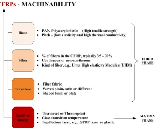
Figure 2.1. 5 Material properties of CFRPs governing the machine ability of CFRPs
Figure 2.1.5 shows the two different phases of material with different properties used
to make CFRPs. Each machining method demonstrated different properties. There are
three main methods to producing carbon fibers. The first method uses polyacrylonitrile
fibers and produces the highest-modulus carbon fiber. The second method is from
mesosphere pitch that produces a higher-thermal carbon fiber. The third method of
producing carbon fiber uses a gas phase and pyrolytic deposition of hydrocarbons.
2.1.2.1 Matrix and Properties
Composite matrix materials are commonly polymers, metals, and ceramics. The most
common of these are polymers; it’s cheap and the structure is more complex than others.
As polymers are the most often used resins in composite matrices while metal and
ceramic are used for specialized applications, this research will focus on the use of
polymers.
2.1.2.1.1 Polymers
Polymers possess an inexpensive complex structure that is easily manufactured at a
and cannot be used in elevated temperatures. Prolonged exposure to ultraviolet light and
some solvents can degrade polymer properties. Generally, polymers are poor conductors
of heat and electricity because of predominantly covalent bonding. However, they are
more resistant to chemicals than metals are. Structurally, polymers are composed of giant
chainlike molecules. Polymerization is the process of joining many monomers together to
form large polymeric molecules.
There are two types of polymerization: condensation polymerization and addition
polymerization (Chawla 2012). Condensation polymerization is a stepwise reaction of
molecules. In each step, a molecule of a simple compound forms as a by-product.
Addition polymerization is generally carried out in the presence of catalysts. In this
process, the monomers do not produce any by-products.
There are also two major classes of polymer that can be produced by either the
condensation or addition polymerization: thermoplastic and thermoset polymers.
Figure 2.1. 6 Possible Arrangements of Polymer Molecules: (a) Amorphous, (b) Semi-crystalline (Chawla 2012)
Thermoplastic polymers soften or melt on heating and are suitable for liquid flow
forming. Its polymer chains are not cross-linked. Thermoplastics can be either amorphous
or semi-crystalline. When the structure is amorphous, there is no apparent order of the
molecules as illustrated in Fig.2.1.6 (a). In fig. 2.1.6 (b), long molecular chains are folded
in a regular manner; the small, plate-like single crystalline regions are lamellae or
crystallites, the crystallites combine together and form spherulites. Some of the most
If the molecules in a polymer are cross-linked in the form of a network, the polymer
does not soften or melt when heating. These polymers are called thermosets. As the
cross-linked molecules cannot slide past one another, the polymer is strong and rigid.
Thermoset composite materials are advantageous for high temperature applications.
Epoxy, phenolic, polyester and vinylester are all thermoset polymers.
Table 2.1.4 shows some thermoplastic and thermoset materials and their properties.
Table 2.1. 4 Typical structural matrix resins (Chawla 2012)
Figure 2.1. 7 Different types of copolymers (Chawla 2012)
Polymers also can be classified by the type of repeating unit. As Figure 2.1.7 shows,
there are three types: random, block, and graft. Each repeating unit forming the polymer
chain is called homopolymer. If polymer chains are composed of two different monomers,
the constructed units are called copolymers.
The chemical resistance of the polymer matrix is better than only carbon fiber and the
toughness and damage tolerance can be controlled by the design of the composite
material. Carbon fiber composites also have dimensional stability which can be designed
for zero coefficient of thermal expansion. In conclusion, carbon fiber composites,
according to their superior performance, are the best choice for automotive and aerospace
2.2 Carbon Fiber Composite Materials
As discussed before, composite materials contain multiple materials blended together.
Among the reinforcements and matrices, a carbon fiber composite has carbon fiber as at
least one of the components. The fiber can be short or continuous, unidirectional or
multidirectional. Commonly, the matrix is polymer, metal, carbon, ceramic, or hybrid
combinations. Furthermore, the matrix is continuous in all directions. Compared with the
matrix, fiber reinforcements are often discontinuous in all directions, which means most
materials have different performance along the various fiber directions, unless the fibers
are three-dimensionally interconnected (Chung 1994).
In section 2.1.2.1.2, carbon fiber was introduced. In carbon fiber itself, the chemical
bonding and Van Der Waals bonding are strong enough to address most mechanical
requirements. Moreover, for fiber composite materials, the high strength and modulus of
carbon fibers makes them much more useful as the reinforcement for the matrix. In other
words, the bonding between fiber reinforcement and matrix play an important role in
material performance. In a unidirectional fiber composite, the longitudinal tensile strength
is quite independent of the fiber-matrix bonding, but the transverse tensile strength and
the flexural strength increases with the effect of fiber-matrix bonding. To further
understand fiber composite materials, classifications of different types of combinations
will be discussed.
As noted before, the matrix material described here only refers to polymer materials.
2.2.1 Fiber Composite Materials Classifications
Just as the polymers can be divided into thermoplastics and thermosets, so can carbon
fiber composites be classified as carbon fiber-reinforced thermoplastics and carbon
fiber-reinforced thermosets. The advantages of the carbon fiber-reinforced thermoplastics
follows (Chung 1994):
(1) Lower manufacturing cost:
No cure
Unlimited shelf-life
Reprocessing possible (for repair and recycling)
Less health risks due to chemicals during processing
Low moisture content
Thermal shaping possible
Weldability (fusion bonding possible)
(2) Better performance:
High toughness (damage tolerance)
Good hot/wet properties
High environmental tolerance
Of course, there are some disadvantages of thermoplastics compared to thermoset
composite materials such as the limitations in processing methods, high processing
temperatures, high viscosities, stiff and dry prepregs, and less developed fiber surface
treatments.
In general, composite materials can be classified by the fibres’ form. In this way, the
carbon fiber polymer-matrix composites can be continuous fiber composites and short
fiber composites. According to the fiber type, continuous fiber composites have
significantly different properties from the short fiber composite mechanically, or even in
their electrical resistivity, thermal conductivity, and other properties. Consequently, the
material that is the focus of this research can be summarized as continuous carbon
fiber-reinforced thermoplastic composite.
2.2.2 Continuous Carbon Fiber Polymer-matrix Composite Properties
high-strength steels. They are all stiffer than titanium. Fatigue resistance and creep
resistance of carbon fiber composites are ideal. Some carbon fiber composites have low
friction coefficients resulting in good wear resistance (Chung 1994).
2.3 Composite Material Process Methods
In this section, some composites manufacturing processes will be introduced,
including traditional and advanced methods. As described before, thermosets and
thermoplastics are the two main classes of polymeric matrix materials. Thus, the process
can be divided into two main categories even though some of the approaches can be used
on both types of polymers.
2.3.1 Processing of Thermoset Matrix Composites
For composite materials having a thermoset matrix, there are many processing
methods such as hand layup and spray techniques, filament winding, pultrusion and resin
transfer molding.
2.3.1.1 Hand Layup and Spray Technique
Hand layup and spray techniques are simple manufacturing processes. As the name
suggests, hand layup composites are created by manually placing the fibers in a mold and
spraying or brushing the resin (commonly is the polyester) on fibers by hand as shown in
Figure 2.3.1. Additionally, with spray-up techniques, resin and chopped fibers are sprayed
together onto the mold surface. In both methods, the layers are formed by hand using
rollers. Mixed fiber and matrix can be completely cured at room temperature or at a
Figure 2.3 1 (a) in hand layup, fibers are laid onto a mold by hand and the resin is sprayed or brushed on (b) in spray-up, resin and fibers (chopped) are sprayed together onto the mold surface (Chawla 2012)
2.3.1.2 Filament Winding
Filament winding is a very versatile technique used for continuous fiber tows or
rovings passing through a resin impregnation bath and wound over a rotating or stationary
mandrel. This kind of approach can produce very large cylindrical like pipes and
spherical vessels, as the winding of the roving can be hoop or helical. Curing of thermoset
resin can be done at an elevated temperature, after which the mandrel is removed. (Figure
2.3.2) (Chawla 2012)
Figure 2.3 2 (a) schematic of filament winding process (b) Schematic of a filament wound pressure vessel with a liner; helical and hoop winding are shown (Chawla 2012)
There are two types of filament winding process. The first process is called wet
polyesters and epoxies with viscosity less than 2 Pa·s (20 P) is applied to the filaments.
Another process is named prepreg winding. The fiber, in this process, will be
preimpregnated by a hot-melt or solvent-dip process. Unlike the wet winding process, the
rigid amines, novolaces, polyimides and higher-viscosity epoxies are generally used. For
the filament winding approach, the void sites are most likely roving crossovers and
regions between layers with different fiber orientations.
2.3.1.3 Pultrusion
The pultrusion process has a continuous molding cycle which requires that the fiber
distribution and the cross-sectional shapes are constant. Low labour cost and consistency
of the product are advantages of the process. Additionally, products like rods, channels,
angle, and flat stock are easily produced. The reinforcements used in this process can also
be different forms such as roved continuous fibers and continuous strand fiber mats. If
using the chopped fiber or chopped strand mat, carrier material is required (Figure 2.3.3)
(Chawla 2012).
Figure 2.3 3 Schematic of the pultrusion process (courtesy of Morrison Molded Fiber Glass Co)
2.3.2 Processing of Thermoplastic Matrix Composites
There are several advangtages and disdavantages of thermoplastic matrix composites
compared to thermoset matrix composites. Chawla (Chawla 2012) summarized some
advantages of thermoplastic matrix composites:
(1) Refrigeration is not necessary with a thermoplastic matrix
(3) Parts can be remolded, and any scrap can be recycled
(4) Thermoplastic matrix composites have better toughness and impact resistance than
thermoset matrix composites.
Disadvantages of thermoplastic matrix composites include:
(1) Processing temperatures are generally higher than those with thermosets.
(2) Thermoplastics are stiff and boardy, i.e., they lack the tackiness of the partially cured
epoxies.
(3) A wish quality composite laminate must have no void. For this reason, there must be
sufficent flow of the thermoplastic matrix between layers and also within individual
tows. The molding cycle time is shorter for thermoplastic matrices than that for
thermoset matrices.
2.3.2.1 Film Stacking
The laminae are stacked alternately with thin films of pure polymer matrix material.
The laminae consist of fibers impregnated with insufficent matrix and polymer films of
complementary weight to give the desired fiber volume fraction of the finished product.
The pressure and temperature must be sufficient to force the polymeric melt to flow into
and through the reinforcement preform. As Darcy’s Law (Chawla 2012) states, increasing
the applied pressure and decreasing the viscosity of the molten polymer can obtain a
better end product.
2.3.2.2 Diaphragm Forming
Diaphragm forming is the sandwiching of a freely floating thermoplastic prepreg
layer between two diaphragms. The air in the gap between the diaphragms will be
evacuated. The thermoplastic laminate is heated above the melting point of the matrix.
The pressure, applied to one side, deforms the diaphragms and forces the material to
thake the shape of the mold. Because the laminate layers are freely floating and very
flexible above the melting point of the matrix, the laminae can be conformed to the mold
the diaphragms stripped off to obtain the resulting compoiste part (Chawla 2012).
2.3.3 Introduction to RTM, Injection Molding, SMC, and LFT-D-ILC
Currently, there are several methods to produce FRP using different kinds of
fiber-reinforced material. One of these processes is Direct Long Fiber Thermoplastic
Molding (LFT-D). In this process, thermoplastic material is directly compounded with
long fibers. There are two direct benefits to using LFT-D: precision of the fiber length,
and determination of the approximate angle of the fiber. In addition, compound properties
can be controlled. Compared to Sheet Molding Compound (SMC) processes for FRP, the
LFT-D results in a lower quality surface finish. However, the processing time for LFT-D
is much shorter and is easier to mold. Furthermore, it is obvious that long continuou
fibers can bring better performance when fiber orientation of the material so greatly
influences the material performance.
2.3.3.1 Resin Transfer Molding (RTM)
Resin transfer molding (RTM) is a closed-mold, low-pressure process for preformed
fiber, such as glass or carbon. The fiber component is placed inside the mold and liquid
resin, such as epoxy or polyester, is injected into the mold by means of a pump.
Reinforcements can be stitched, but more commonly they are made into a preform sheet
or desired shape. During injection of the polymer matrix the shape is already dictated by
the shape of the mold. The completed composites are able to cure and form as a solid in
the mold during the process.
For this process, the polymer viscosity should be low enough for the fibers to be
wetted easily and the polymer itself to flow smoothly.
RTM has its own advantages as follows (Chawla 2012):
(1) Easier to obtain large, complex shapes, and curvatures.
(2) Processing has a higher level of automation than others.
Fiber volume fractions can be achieved as high as 65% by using woven, stitched, or
braided performs.
The process uses a closed mold, resulting in reduction of styrene emissions.
Generally, RTM produces much fewer emissions compared to hand layup or spray-up
techniques.
Mold design is a critical element in the RTM process. Sometimes, the fibrous
preform is preheated and the mold has built-in heating elements to accelerate the process
of resin curing. Resin flow and heat transfer are analyzed numerically to obtain an
optimal mold design. Usually, the automotive industry uses RTM because it is a
cost-effective, high volume process.
2.3.3.2 Injection Molding
Because thermoplastics get soft when heated, melt flow techniques of forming can be
used. Injection molding is one of these technologies. Generally, short fiber reinforced
thermoplastic composites can be produced by reinforced reaction injection molding
(RRIM) which is actually an extension of the reaction injection molding (RIM) of
polymers. During RIM, two liquid components (resin and short fiber) are pumped into a
mixing head at high speed and pressure and then they enter a mold together where the two
components react to polymerize rapidly. During RRIM, short fibers (or fillers) are added
to one or both of the components. The lengths of fiber, added into the mold, are generally
short and the specifications are limited by the viscosity. Because a certain minimum
length of fiber, the critical length, is required for effective fiber reinforcement, RRIM
additives are fillers rather than reinforcements. Most RIM and RRIM applications are in
the automotive industry as welle (Chawla 2012).
2.3.3.3 Sheet Molding Compound (SMC)
The additives consist of fine calcium carbonate particles and mica flakes. Sometimes,
for lower density, calcium carbonate powder is substituted with hollow glass
vinylester. Both reduction techniques for density and weight are costly. Generally, in
practice, some auto body parts, such as bumpers, beams, and radiator support panels, are
produced by SMC. However, SMC has longer cure times of up to two days (Chawla
2012).
Currently, there is a process called Direct Sheet Molding Compound (D-SMC). The
advantage of D-SMC is not only better material properties, but also reduced processing
time, dramatically increasing efficiency and decreasing cost for industry.
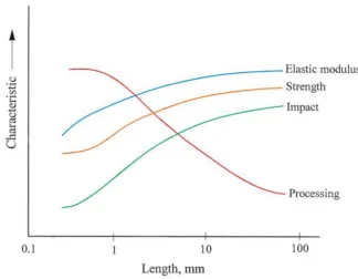
2.3.3.4 Long Fiber Thermoplastic Compression Molding (LFT)
Long Fiber Thermoplastic Compression Molding, as the name implies, refers to
processing composites using a thermoplastic matrix with fibers greater than 10 mm in
length. As Figure 2.3.4 shows, the length of the fibers can determine the mechanical
properties of composite materials.
Figure 2.3 4 Variation of Some Mechanical Properties of a Composite as a Function of Fiber Length (Chawla 2012)
Figure 2.3.4 shows advantages of increased fiber length, illustrating why there is a
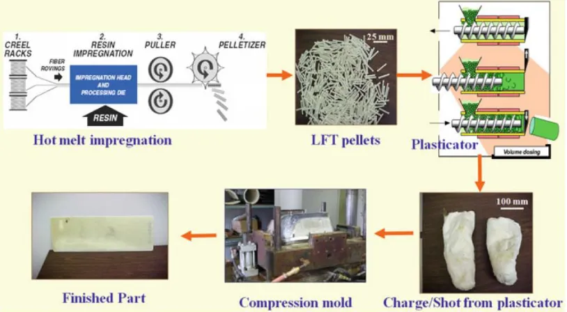
LFT is shown in Fig. 2.3.5. The critical step in processing LFTs is the production of
continuous fiber reinforced rods or tapes from which long fiber pellets are cut.
Figure 2.3 5 Extrusion/compression molding process for making long fiber reinforced thermoplastic (LFT) composites. Hot melt impregnation of fibers is used to produce tapes, rods or long pellets of LFT. Pelletized
LFT material is fed into an extruder or plasticator. (Chawla 2012)
In this process, continuous fiber tows are first passed through a bath of molten matrix
and then through a die for shaping into a rod or ribbon, followed by passage through a
chiller for cooling. The final stage involves a puller/chopper; the puller pulls the tow at
the desired speed as soon as the chopper cuts the continuous, impregnated tow to desired
length of pellets suitable for use in an extruder and compression mold. The long fiber
pellets are suitable for the conventional injection molding process, injection compression
molding, as well as the extrusion compression molding processes. The LFT pellets made
by hot melt impregnation are fed into a plasticator where they are metered into a barrel,
heated above the melting point of the thermoplastic resin, and the mixture of polymer
plus fiber flows through a low shear plasticator to form a molten charge. The molten
charge coming out of the plasticator resembles cotton candy and is quickly transferred to
a heated mold where it is compressed in a closed tool (generally, a high tonnage press).
2.3.4 LFT-D Processes
There is another commercial process called, LFT-D-ILC (direct long-fiber
thermoplastic in-line compounding) or LFT-D, which has been used to make LFT
composites consisting of styrene copolymers/glass fibers. Polypropylene has also been
used as a thermoplastic matrix in this process. Essentially, it is an extrusion/ compression
molding process. The distinctive feature of the LFT-D-ILC process is that the long fiber
composite is produced directly from the basic materials. The polymer matrix material and
any modifiers/additives are mixed and melted in a compounding extruder. This mixture is
combined with the reinforcing fibers in a twin screw extruder (Krause et al. 2003). The
special screw-design disperses the fibers in the matrix and further fiber breakage is
avoided. The extruder machines work continuously and produce a continuous long fiber
reinforced extrudate, which is cut into pieces of the desired length and is then directly
compression molded.
LFT-D-ILC is a technology useful in establishing long-fiber thermoplastic material
processing in the automotive industry. The aim is to produce lighter and stronger
composite material as compared to metal. The LFT-D-ILC technology produced by
Dieffenbacher consists of two technologies: the hydraulic press and LFT-D line.
The LFT-D line produces charges for pressing. These charges consist of mixed
melted polymer and preheated fibers. The hydraulic press is a high-speed compression
mold in which the charge is placed. In practice, the hydraulic press can fabricate a
Figure 2.3 6 Process scheme of LFT-D line
As Figure 2.3.6 shows, throughout the fiber feeding section, the continuous fiber is
fed into the extruder from the fiber tow, where it is mixed with the polyamide. The
polyamide, coming from the dosing unit, is melted as it passes through the heated
extruder. At the second extruder, the fiber is mixed in a set direction with the melted
polyamide and the charge is produced for the press. The charge goes in the oven on a
conveyor, and then charge put into the press machine where the panel is produced.
Figure 2.3 8 Charge produced by LFT-D prepared for press
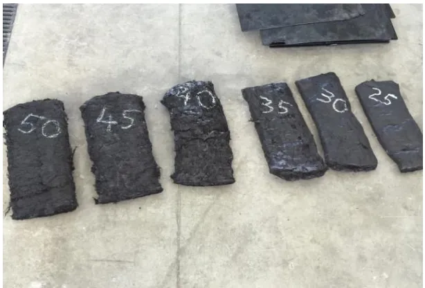
Figure 2.3 9 Test panels produced by LFT-D process
Figure 2.2.7 shows fiber tow on rovings as it is fed into the LFT-D line. Generally,
continuous long fiber (fiber tow) is easier for feeding. Unless the fiber is fed smoothly
into the machine, the mechanical properties cannot be guaranteed. Figure 2.3.8 shows the
presscharge which is produced by the LFT-D line. The weight and the fiber volume of the
charge can be set and determined by the machine. Commonly, using an oven to maintain
Figure 2.3.9, the black panel is the material produced by the LFT-D trial. These panels
are also the test panels from which data was measured for the current research.
2.4 Introduction to Neural Networks
2.4.1 Introduction to Neural Networks
Artificial neural networks (ANNs), in machine learning and cognitive science,
evolved from the basic information processing methods found in the brain. The ANN is a
model of statistical learning algorithms to estimate or approximate a related function by
examining patterns in a large amount of data. Generally, it is a black-box tool used to
describe the relationship between input and output data sets.
Derived from the biological central nervous system in the brain, the basic units are
called neurons and connect to each other to form a network. Generally, an artificial neural
network has three types of layers to imitate animals’ feedback processes: an input layer,
hidden layers, and an output layer. The input and output data are held in the input and
output layers respectively. The hidden layers use transfer functions to connect the input
and output layers (Samarasinghe 2006), with relative importance achieved by weighting
the various paths from input through to the output layers with weights and bias values that
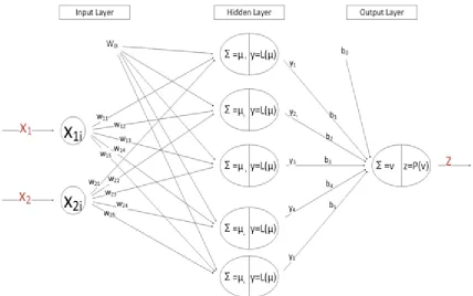
will be described (see Figure 2.4.1).
In the general case, the full process of neural network development includes training,
validation, and testing. Before training a neural network, the first key step is to select a
proper network configuration. Figure 2.4.1 shows a 2-5-1 feed-forward backpropagation
neural network, as an example, to introduce the neural network development process. A
2-5-1 network is named according to the number of neurons in the input, hidden, and
output layers, respectively.
So far, the ANN has a complete basic structure: the neurons in different layers are
obvious that the ANN can be represented by different numbers of neurons, layers, and
combinations of transfer functions. Figure 2.4.1 is the structure of a one hidden-layer
feed-forward backpropagation neural network (section 5.2.1 describes the feed-forward
backpropagation neural network).
Figure 2.4 1 A 2-5-1 backpropagation feed-forward neural network configuration
Between the input and hidden layers, and between the hidden and output layers,
weights connect each pair of neurons (w11, w21, b1, b2, etc.). Bias values at each neuron act to shift the summed weighted inputs before being passed to the transfer function (w0i and
b0). Both weights and biases are key parameters of neural network that are adjusted
during network training.
In the first layer (input layer): x1 and x2 represent the input data (i.e. two input
variables). As soon as the inputs are transferred to the hidden layer, they are multiplied by
the connecting weights and a bias added to form variable μi, that are input to the hidden
layer neurons:
In this equation, μi represents the weighted sum of inputs to the ith hidden layer neuron. (n
is the number of neurons in hidden layer). Then, the μi pass through the ith neuron transfer
function (also referred to as activation function) denoted yi=Li(μi). Various transfer functions can be used for nonlinear neurons in a neural network, as shown in Figure 2.4.2
(Samarasinghe 2006).
Figure 2.4 2 Some Nonlinear Neuron Transfer Functions: (a) Logistic, (b) Hyperbolic-Tangent, (c) Gaussian, (d) Gaussian Complement, (e) Sine Function (Samarasinghe 2006)
The functions shown in Figure 2.4.2 are vital to neural information processing with
their special characteristics. These functions are nonlinear, continuous, bounded functions.
Their nonlinear character enables the neural network to model nonlinear relationships
between inputs and outputs. Continuity of the function makes it possible to adjust the
weights during the error backpropagation process.
There are three main classifications of nonlinear transfer functions: sigmoid functions,
Gaussian functions, and sine functions. Sigmoid functions are a family of S-shaped
functions. The sigmoid functions include the logistic function and hyperbolic tangent
function.
The logistic function has a wider range (i.e. [-1, 1]) than that of the hyperbolic
tangent (i.e. [0,-1]). The formulation of the logistic function is
𝑦 = 𝐿(𝜇) =1+𝑒1−𝜇 (2-2)
Where e is the base of natural logarithm, equal to 2.71828. Another commonly used sigmoid function is the hyperbolic tangent function,
Gaussian functions also include two commonly used functions: standard normal curve
and Gaussian complement.
𝑦 = 𝑒−𝜇2
(Standard normal curve) (2-4)
and
𝑦 = 1 − 𝑒−𝜇2
(Gaussian complement) (2-5)
Both of these functions have range [0, 1]. The standard normal curve peaks at μ=0 and Gaussian complement assumes a value of zero when μ=0.
In general, the sigmoid function, Gaussian functions and sine functions have
additional variations. In the current research, sigmoid functions are applied due to their
popularity. In MATLAB’s neural network toolbox, there are three commonly used
transfer functions for feed-forward networks (introduced in section 5.2.1):
Logsig function
𝑦 = 1/[1 + 𝑒𝑥𝑝(−𝑥)] (2-6)
Tansig function
𝑦 = 2/[1 + 𝑒𝑥𝑝(−2𝑥)] − 1 (2-7)
Purelin function
𝑦 = 𝜇 (2-8)
It is obvious that in the input-hidden layer, the logsig function and tansig function are
the same as function (2-2) and function (2-3) when x=µ. These two functions are used to implement in these research as the neural networks are developed and evaluated.
The purelin function is often used in the hidden-output layer to calculate the output.
Actually, tansig and logsig functions can be applied in the output neurons as well.
However, these two functions make the calculations more complicated without increasing
the accuracy (J. Xu 2007). If it becomes necessary to improve the network accuracy, it’s
more common to increase the number of hidden layers instead of using nonlinear
functions in the output neurons.
hidden-neuron output yi. The function can be written as
𝜈 = 𝑏0+ 𝑏1𝑦1+ 𝑏2𝑦2+ 𝑏3𝑦3+ 𝑏4𝑦4+ 𝑏5𝑦5 (2-9)
Where b0 is the bias weight for output neuron and bj are the weights for the hidden-output neuron weight. If the purelin function is used in the output layer,
𝑧 = 𝜈 (2-10)
For the general cases, the weighted sum ν comes from the hidden neurons and can be represented by y and the output z as:
𝜈𝑘 = 𝑏0𝑘+ ∑ 𝑏𝑗𝑘𝑦𝑗𝑘 𝑙
𝑚 𝑗=1 𝑘=1
(2-11)
𝑧𝑘 = 𝜈𝑘 (2-12) Where bjk is the weight linking hidden neuron output yjk and the kth output neuron. l is the number of hidden neurons and m is the number of network outputs.
For the example 2-5-1 backpropagation feed-forward neural network, the neural
network variables can be written as shown in equations (2-13) to (2-17).
Input-hidden layers:
𝜇𝑖 = 𝑤1𝑖𝑥1 + 𝑤2𝑖𝑥2+ 𝑤0, i = 1 to 5 (2-13)
𝑦𝑗 =1+𝑒1−𝜇 , j = 1 to 5 (2-14)
or
𝑦𝑗 =1+𝑒1−𝑒−𝜇−𝜇 , j = 1 to 5 (2-15)
Hidden-output layers:
𝜈 = 𝑏0+ 𝑏1𝑦1+ 𝑏2𝑦2+ 𝑏3𝑦3+ 𝑏4𝑦4+ 𝑏5𝑦5 (2-16)
𝑧 = 𝜈 (2-17)
Where z is the output of the neural network. During training, z will be compared with the target data t to get the error in network prediction.