Performance Analysis of TCP over Wired and Wireless Network

(1)

XINBING WANG. Performance Analysis of TCP over Wired and Wireless Networks. (Un-der the direction of Professor Do Young Eun.)

Transmission Control Protocol (TCP) currently accounts for about 90% applica-tions and 80% data of network traffic, and plays the dominant role in Internet transmission. In this dissertation, we present three studies of TCP performance over wired and wireless networks. In the first study, we mainly focus on the stability of TCP/AQM (Active Queue Management) systems for wired network environment. In particular, we study the local and global stability of TCP-newReno/RED under many flows regime. By using a normal-ized discrete-time model, which is simple, we analyze the global stability in a very efficient manner, and the results show that by properly choosing RED parameters, we can always make the TCP-newReno/RED system globally stable.

The second study concerns the TCP performance when the buffer size is scaled up differently from the traditional one at a link with large capacity shared by many flows. Specifically, we consider the buffer size chosen on the order of (Nα_{) (0}_{< α <}_{1), where}_N

flows share the link of capacity O(N). We then develop a doubly-stochastic model for a TCP/AQM system with many flows by taking into account the packet-level dynamics over fine time scales. We show that, under our scale, the system always performs well in the sense that the link utilization goes to 1 and the loss ratio decreases to zero as the system sizeN increases. We verify our results using extensivens-2 simulations.

(2)

by

Xinbing Wang

A dissertation submitted to the Graduate Faculty of North Carolina State University

in partial fulfillment of the requirements for the Degree of

Doctor of Philosophy

Electrical and Computer Engineering

Raleigh

2006

Approved By:

Dr. Arne Nilsson Dr. Peng Ning

Dr. Wenye Wang Dr. Robert Martin

(3)

(4)

Biography

(5)

Acknowledgements

First and foremost, I want to thank my advisor, Professor Do Young Eun, who led me into this exciting area of networking performance analysis. As his first Ph.D. student, I am very fortunate to share more opportunities to work closely with him. I cannot imagine how much time and patience he spent to train such a ‘stubborn’ student like me and explain the problems, ideas, thinking, insights and the way how to be a genuine researcher, which becomes the most valuable experience in my life. I am privileged to have such a wonderful advisor, who is always enthusiastic, inspired, patient, helpful and encouraging. I cannot overstate my gratitude and appreciation for his encouragement and support. All I can say is that I can hardly ask for any more from an advisor, I will also try to be such a devoted teacher and a great mentor to my future students, I will make sure that when they write acknowledgements, the thanks also go to Professor Eun. At the same time, I would like to thank my co-advisor Professor Wenye Wang for her great patience and the extensive training, without which I could not have finished my Ph.D. study. I would also give many thanks to Professor Peng Ning, Professor Arne Nilsson and Professor Robert Martin for teaching me important research tools and for their kind guidance. In addition, I am particular grateful to Professor Bibhuti B. Bhattacharyya in Statistics Department and Professor Min Kang in Mathematics Department, who taught me a rich of modern probability and stochastic processes theory that will definitely benefit me in the rest of my life. Thanks also to Professor Xiuli Chao and Professor Shu-Cherng Fang in Industry Engineering Department for enlightening me with queueing theory and programming theory, respectively.

Besides these professors, I feel very lucky to meet my friends like Tie Liu, Peng Xu, Xiang Zhou, Haidong Guo, Tiejun Li, Dingbang Xu, Pan Wang, Hua Li, Chuan Lin, Yipeng Yang and many others, who give a lot of help to me or have valuable discussions with me. Also, I am grateful to my officemates including Yuh-Ming Chiu, Han Cai, Sungwon Kim, Terrence A. Vanvalkenhoef, Wei Liang, Ming Zhao, Fei Xing, Yi Xu, Jangeun Jun, Rong Peng and Suyoung Yoon, etc.

(6)

List of Figures

2.1 Performance: Tuning TCP buffers and parallel streams [48]. . . 13

2.2 Performance Comparison: Aggregate Bandwidth. Auto: the proposed scheme; Hiperf: Tuning by Hand; Default: Default setting by NetBSD [176]. . . 14

2.3 Performance Comparison: Peak usage of memory. Auto: the proposed scheme; Hiperf: Tuning by Hand; Default: Default setting by NetBSD [176]. 15 2.4 Illustration: Traditional TCP and STCP [106]. . . 16

2.5 Fairness of HSTCP over regular TCP [70]. . . 17

2.6 TCP Fairness [197]. . . 18

2.7 Fairness of TCP SABUL [78]. . . 21

2.8 TCPWestwood and TCP-Reno: Throughput vs. bottleneck bandwidth [144]. 22 2.9 TCPWestwood and TCP-Reno: Throughput vs. bottleneck buffer size [144]. 23 2.10 Interplanetary Internet [8]. . . 23

2.11 State Transition Diagram [8]. . . 24

2.12 Three Types of Loss in Cellular Networks. . . 25

2.13 Two State Markov Chain for Loss Channel [83]. . . 25

2.14 Network Scenario for 802.11b WLAN [29]. . . 26

2.15 Three State Markov Chain for Error [29]. . . 26

2.16 An Example of Bandwidth Variation over time [20]. . . 27

2.17 An Example of Round Trip Time Variation over time [20]. . . 27

2.18 Illustration of TCP Connection Establish [37]. . . 32

2.19 Throughput Comparison of Tahoe, Reno and Sack for (a), (b) correlated and (c) independent losses [154]. . . 35

2.20 Performance of RED compared to Droptail. First column is droptail; Second column is RED without ECN; Third column is RED with ECN [69]. . . 37

2.21 REM Marking Function compared to RED [18]. . . 38

2.22 AVQ: Virtual Queue is not full [122]. . . 39

2.23 AVQ: Virtual Queue is full [122]. . . 40

2.24 AVQ Algorithm in Pseudocode [122]. . . 40

2.25 AVQ Performance compared to RED, PI, REM, GKVQ with regard to Av-erage Queue Length [122]. . . 41

2.26 BLUE: Core Algorithm in Pseudocode [60]. . . 42

(10)

2.28 PI Controller [35]. . . 44

3.1 The stability convergence with the number of flowsN . . . 48

3.2 An Example to illustrate the relationship between RED slope ρ and RTT: the round trip physical propagation delay is 200 ms; capacity for each flow C is 10 packets/sec. . . 49

3.3 System model and RED algorithm. . . 52

3.4 Model comparison when the system is unstable. . . 55

3.5 Model comparison when the system is stable. . . 56

3.6 Model comparison when the system is stable. . . 57

3.7 The Bound of Q(t) and W(t). . . 62

3.8 Example I: the stable region of Q(0) and W(0) withQ(∞) = 1.2764,W(∞) = 12 for ∆q= 0.3,0.4,0.5,0.6. . . 64

3.9 Example II: the stable region of Q(0) and W(0) with Q(∞) = 3.8237, W(∞) = 6.70 for ∆q= 0.05,0.07,0.08,0.1. . . 65

3.10 The impact ofband ato the system stability with C= 20, ρ1 = 0.01. . . . 71

3.11 The impact ofband ato the system stability with C= 20, ρ1 = 0.01. . . . 72

3.12 The comparison of stability region and decomposition for Heterogenous RTTs. 78 3.13 The average window size and normalized queue-length under different number of flowsN. . . 81

3.14 The average window size and instantaneous queue-lengthQN_{(t) with different} initial window size W(0) and under fixedQ(0) = 5. . . . 82

3.15 The decomposition for heterogenous RTTs. . . 83

4.1 Examples of marking functions with aggressive marking scale ofNα_{. . . . .} ₈₆

4.2 Queue-length fluctuation using ns-2: (a) stable queue; (b) unstable queue with aggressive marking; (c) comparison of (a) and (b) over the same y-axis. 88 4.3 The CLT argument in [17] foro(N0.5_{). . . .} ₉₀

4.4 The CLT argument for our scheme in [51] foro(Nα_),₀_{< α <}_{0.5. . . .} ₉₁

4.5 Homogeneous RTTs: Performance metrics with increasing number of flows (N) for fixed α= 1. . . 93

4.6 Homogeneous RTTs: Performance metrics with increasing number of flows (N) for fixed α= 0.2. . . 94

4.7 Heterogeneous RTT: Performance metrics with increasing number of flows, N for fixedα= 1. . . 96

4.8 Heterogeneous RTTs: Performance metrics with increasing number of flows (N) for fixed α= 0.2. . . 97

4.9 Webmice traffic: Performance metrics with increasing number of persistent flows,N for fixedα= 1. . . 98

4.10 A mixture of short- and long-lived flows: Performance metrics forα= 0.2 as the number of persistent flows (N) increases. . . 99

4.11 Simulation topology: multiple bottleneck links with heterogeneous RTTs. . 100

(11)

5.1 The TCP AIMD algorithm under a constant loss rate. . . 104

5.2 The system model and the interaction between call level and packet level. . 105

5.3 The algorithm for the base station to obtainp(t). . . 112

5.4 The rate control scheme based onpi(t): stochastic packet dropping. . . 114

5.5 Stochastic admission control for a system with a queue. . . 115

5.6 M/M/1 model of packet arrival/serivce process. . . 117

5.7 The system model with high priority queue and the priority weight function with queue length: g₁(x) and g₂(x) are monotone nondecreasing functions withg1(x0)> g2(x0), ∀x0 . . . 119

5.8 The blocking probability comparison for with and without TCP AIMD control.130 5.9 The throughput comparison for with and without TCP AIMD control. . . . 131

5.10 The link utilization comparison for with and without TCP AIMD control. . 132

5.11 The performance metrics of TCP-AIMD aware with the two-dimensional in-crease of both λ1 and λ2. . . 133

5.12 The blocking probability of Class 1 for different TCP AIMD control: p1 = 0.1667, p2 = 0.0938, p3 = 0.0600, p4 = 0.0417 corresponds to E{TCP}1 = 3, E{TCP}2= 4, E{TCP}3 = 5, E{TCP}4= 6 pkt/sec, respectively. . . 134

5.13 The blocking probability of Class 2 for different TCP AIMD control: p1 = 0.1667, p2 = 0.0938, p3 = 0.0600, p4 = 0.0417 corresponds to E{TCP}1 = 3, E{TCP}2= 4, E{TCP}3 = 5, E{TCP}4= 6 pkt/sec, respectively. . . 134

5.14 The throughput of Class 1 for different TCP AIMD control: p1 = 0.1667, p2 = 0.0938, p3 = 0.0600, p4 = 0.0417 corresponds to E{TCP}1 = 3, E{TCP}2 = 4, E{TCP}3= 5, E{TCP}4 = 6 pkt/sec, respectively. . . 135

5.15 The throughput of Class 2 for different TCP AIMD control: p1 = 0.1667, p2 = 0.0938, p3 = 0.0600, p4 = 0.0417 corresponds to E{TCP}1 = 3, E{TCP}2 = 4, E{TCP}3= 5, E{TCP}4 = 6 pkt/sec, respectively. . . 136

5.16 The link utilization for different TCP AIMD control: p1 = 0.1667, p2 = 0.0938, p3 = 0.0600, p4 = 0.0417 corresponds to E{TCP}1 = 3, E{TCP}2 = 4, E{TCP}3= 5, E{TCP}4 = 6 pkt/sec, respectively. . . 137

5.17 The performance comparison under different distributions of transmission time: Exponential distribution; Lognormal distribution; Uniform distribu-tion. p= 0.1667. . . 138

5.18 The link utilization for different arrival rate: (i) fixedp(t) = 0.1667; (ii) fixed p(t) = 0.0238; (iii) dynamicp(t)∈[0.0234,0.1667]. . . 139

5.19 The link utilization for different arrival rate:(i) fixedp(t) = 0.1667; (ii) fixed p(t) = 0.0238; (iii) dynamicp(t)∈[0.0234,0.1667]. . . 140

5.20 The link utilization for different arrival rate:(i) fixedp(t) = 0.1667; (ii) fixed p(t) = 0.0238; (iii) dynamicp(t)∈[0.0234,0.1667]. . . 141

5.21 The link utilization for different arrival rate: (i) fixedp(t) = 0.1667; (ii) fixed p(t) = 0.0238; (iii) dynamicp(t)∈[0.0234,0.1667]. . . 141

(12)

(13)

List of Tables

2.1 Design of Reno, HSTCP, STCP and FAST [100] . . . 19

2.2 Equilibrium Transmission Rate [100] . . . 19

2.3 TCP Header Checksum Option [25]. . . 28

2.4 TCP Header Checksum ACK Option [25]. . . 28

3.1 Parameters for model comparison . . . 54

3.2 Simulation Parameters . . . 79

4.1 Performance Comparison of the queues in Figure 3.5. . . 88

4.2 AQM parameters forns-2. . . 92

(14)

Chapter 1

Introduction

Currently, most of today’s Internet traffic are carried out by Transmission Control Protocol (TCP) [91], which accounts for 90% applications and 80% data. As the network evolves, many improvements and modifications are proposed to make TCP meet various requirements such as the environment of high-bandwidth delay product or over wireless links [166, 48, 94, 176, 10, 1, 179, 70, 65, 66]. TCP becomes the de-facto standard for reliable transmission protocol and this situation is expected to last in the foreseeable future. Therefore, it would be important and interesting to understand the underlying schemes regulating TCP behaviors.

(15)

one way or the other.

On the other hand, due to the enormous success of TCP in the wired network [166, 48, 94, 176, 65, 66], it is naturally applied to a wireless environment to obtain the reliable end-to-end transmission. Extensive research has been conducted to make the TCP over wireless feasible such as ATCP [132], M-TCP [32], W-TCP [165], ATP [181], I-TCP [24], and significant efforts have been made to improve the performance of TCP in a wireless link (either infrastructure or ad-hoc mode) [144, 80, 84, 73, 150].

1.1 Motivation

Recently, the researchers intent to explain the TCP the behavior with rigorous approach, rather than test their ideas and algorithms only with simulators, for example NS2. More importantly, theoretical analysis may shed the insight on understanding the underlying reasons of TCP behavior. This research focuses on theoretical analysis of TCP on both wired and wireless networks.

We should admit that the topic of performance analysis of TCP over wired and wireless is too abroad to be accommodated into one thesis work. The three problems investigated in this thesis work may seems to be in an ad-hoc fashion. However, as we shall see, there still exist some connections between the following three pieces of work. In fact, the first work and the second work treats a same problem from two different perspectives, i.e., classical control point of view and modern stochastic control point of view. The third piece of work tries to treat the TCP over wireless network issue from a new angle, i.e., from the resource allocation or admission control perspective. Instead of thinking of one particular flow, we look at the TCP flows sharing a access base station or access point, and studies the multiplexing behavior among all the flows. As we shall see, by intensionally controlling transmission rate of the TCP flows, we can improve the system performance from call admission control point view.

1.1.1 TCP Stability Analysis

(16)

Ac-cording to [138], an unstable TCP/AQM system may increase delay and jitter, which can be detrimental to some delay-jitter sensitive applications, and cause link under-utilization. The existing research on stability of TCP/AQM can be broadly classified into two groups: local stability and global stability.

The local stability is obtained by first linearizing the system around its equilibrium point. Then, by applying the Nyquist theorem to that linearized system, one can have a criterion for the local stability of the system [137, 36, 34, 35, 116]. However, due to the linearization involved, the local stability criterion is applicable only when the system operates near its equilibrium point. If the system operates on a region far away from its equilibrium point, then the nonlinear components may kick in and make such a linear approximation inaccurate. We define astability region of a system by a set of initial points, from which the system eventually converges to its equilibrium point. Then, for a locally stable system, this stability region is usually small and limited around the equilibrium point. On the other hand, the global stability requires that starting fromanyinitial points (not limited to the points near the equilibrium point), the system eventually converges to the equilibrium point. Obviously, the global stability implies the local stability. In general, the global stability is obtained by properly constructing a Lyapunov function [163, 164, 12, 13, 126, 194, 45, 160, 193, 158]. In [45], the authors present a criterion for the global stability of a congestion controller with a single link and a single flow. Further, they show that the global stability criterion for a system with many identical flows sharing a bottleneck link converges to that of a single flow [43]. In other words, the condition for global stability with a single flow can be applied to the case of multiple flows as well.

Although the existing results regarding stability reveal valuable insight into the system design, they have their own limitations. For local stability, it is mostly applied to a system with TCP-Reno [138, 34, 36] instead of TCP-newReno, which is an improved version of Reno and widely deployed in practice. The major difference between TCP-NewReno and TCP-Reno is that for TCP-Reno, multiple packet losses or packet marks within one round trip time (RTT) results in multiple reductions of window sizes, while for TCP-newReno, only one reduction of window sizes is incurred (see [68] for more details). To the best of our knowledge, there is no result regarding the stability criterion of TCP-newReno under many flows.

(17)

consider a large system where the number of flows is hundreds or thousands level. According to [72], the core router is shared by more than 10,000 flows, and we show that for such a large system, the local stability criterion is different from that of a relatively small system. For example, in a small system, the long RTT of a single flow will affect the stability criterion [138]. However, for a large system, we will show in this paper that the RTT for a single flow or a small number of flows will not make any impact on the stability of the system as a whole.

As to the global stability, the AQMs studied in the literature are mostly limited to rate-based marking schemes [43, 45], and not applicable to any other popular queue-based marking schemes such as RED [69]. Still, to the best of our knowledge, there has been no result about the global stability of a TCP-newReno/RED system with many flows. This is mainly due to the following two reasons. First, as the network evolves, the core router is shared by increasingly large number of flows. Since each flow has its own window size dynamics, it becomes more difficult to find an appropriate Lyapunov function for such a system with many flows. Second, the packet marking function for RED is a non-linear (usually piecewise-continuous) function, and this makes any theoretical analysis formidable. All the above observations become our motivation and the techniques to address these problems are provided in Chapter 3.

1.1.2 TCP Performance under a Large Scale

(18)

of Lyapunov) [148, 86, 36, 157, 190, 139, 104, 121, 124], the impact of feedback delay and random noise [101, 178, 203], and the asymptotic behavior of the system when the number of users is large [87, 178, 44, 186, 183].

However, one thing is common in all of the above. The stability analysis and all the design guidelines have been made by focusing only on the dynamics over a series of RTTs, where all the packet-level behaviorwithin each RTT are “averaged out” and lumped into a single quantity such as the window size or the transmission rate of each user per RTT.1_Such an abstraction has been extremely useful for the analysis and control of large networks. For example, when there areN flows with capacityN C and linear scaling (O(N)) is employed for the buffer size and AQM (e.g., all the buffer thresholds for packet marking areO(N)), it has been shown that the system dynamics can be described by the normalized version of the system [87, 186] via the law-of-large-numbers type of arguments. Also, by applying standard techniques from traditional control theory, several stability criteria were obtained in terms of parameters of the normalized system [46, 178, 139]. The main underlying idea behind these results would be the notion of ‘first-order’ principle; all the first-order behavior (or mean behavior) of the system can be captured through the ‘normalized’ system, and any other second-order dynamics over finer time scales will not impact the first-order rule provided that the averaged behavior remains the same.

However, such an approach based on the mean behavior of the system (or on averaged quantities) can be fallible and may pose severe limits on our ability to obtain optimal design guidelines for large-bandwidth systems. Our observation is that, when the system is large with many flows, there will be a large number of packets coming from different sources per RTT and their dynamics in time (i.e., random arrival instants) often become too rich to be captured by such a single (averaged) quantity. For instance, if we look back on the issue of buffer sizing for large systems and demonstrate that TCP/AQM systems work well with all the desirable performance even under a much smaller buffer size and corresponding AQM scale, which as we will show would make the system linearly unstable and thus has been ‘prohibited’. Specifically, we present an example of a TCP/AQM system such that, as the size of the system increases, the performance metrics approach to the optimal case (e.g., 100% throughput, zero loss ratio, etc.) while the system is becoming more unstable (in

1_{An exception is in [47] where packet arrivals within an RTT is explicitly modeled. However, only two}

(19)

the sense of Lyapunov), implying possible performance degradation. While our extensive simulation results to shows that the system always performs well in the sense that the link utilization goes to 1, the queueing delay goes to zero and the loss ratio decreases to zero as the system sizeN increases.

We address this counter-intuitive discrepancy in Chapter 4.

1.1.3 TCP Performance over Wireless Networks

Due to the enormous success of TCP in the wired network [166, 48, 94, 176, 65, 66], it is naturally applied to a wireless environment to obtain the reliable end-to-end transmis-sion. Extensive research has been conducted to make the TCP over wireless feasible such as ATCP [132], M-TCP [32], W-TCP [165], ATP [181], I-TCP [24], and significant efforts have been made to improve the performance of TCP in a wireless link (either infrastructure or ad-hoc mode) [144, 80, 84, 73, 150]. A key feature of TCP congestion control is so called Additive-Increase-Multiple-Decrease (AIMD) algorithm. If there is no packet loss within the current round trip time (RTT), the window size increases by one during the next RTT; Otherwise, the window size decreases by half. Even though the existing literature regard-ing TCP over wireless may differ in different aspects, they share a same TCP essential congestion control algorithm, i.e, AIMD that determines the packet-level TCP dynamics.

In this thesis, we show that such AIMD algorithm plays an important role in affecting the future switched wireless networks such 3G and 4G. Since the packet-switched technology yields more efficient utilization of the scared wireless resource than that of circuit-switched networks, the future 3G and 4G wireless network will be packet-based networks [90, 31, 88, 2] and this is especially true for 4G system 2_{. In a packet-switched} wireless networks, two level performance metrics come into the picture of Call Admission Control (CAC): (i) call level parameters: call blocking probability and handoff dropping probability; (ii) packet level parameters: packet loss probability and link utilization.

Traditionally, CAC schemes deal with call level performance metrics only: call blocking probability and handoff dropping probability [191, 192, 9, 129, 98, 7, 52, 89]. In [130], the admission control algorithm for integrated voice and data traffic is proposed and analyzed. The idea is based on completed sharing method, where the channels within the cell are shared by all the traffic, rather than reserved for a specific class. The

(20)

thors demonstrate that the proposed scheme achieves both service guarantee and service differentiation for voice and data with better bandwidth utilization. In [9], user mobil-ity is considered by the CAC scheme with arbitrary call-arrival rate, which requires the global information on the call arrival process and user mobilities. The proposed scheme is analyzed in terms of a more realistic network topology and their results show that the CAC algorithm achieves high throughput with guaranteed Quality of Service (QoS) and call blocking probabilities. In [129], the mathematical model for on/off traffic model is obtained for a cellular networks provisioning voice and best-effort data service. The traffic is charac-terized by a three-dimensional birth-death model that effectively captures the complicated interaction between on/off voice traffic and best-effort data traffic under a complete sharing situation. The close form for the performance metrics are derived and the minimum amount of resources to guarantee the required QoS is obtained.

All these traditional CAC schemes are limited to the call level performance. Re-cently, packet level performance is taken into account by [75, 202, 201]. The authors propose an efficient CAC scheme for heterogeneous services in wireless ATM networks in [202, 201]. The packet level constraints such as delay and jitter are incorporated into the scheme to guarantee the predefined QoS. A higher priority is assigned to handoff calls to improve the handoff dropping probability by reserving certain amount of bandwidth for potential hand-off calls and such guard-channel like idea is widely applied to the CAC field as in [52, 89]. The simulation results indicate that the proposed CAC scheme can achieve both packet level and call level performance in terms of link utilization and handoff dropping proba-bility. Further in [75], the authors claim that they can even totally remove the handoff dropping event, which is quite desirable from the CAC point of view. The idea is that as long as a handoff call arrives, the system admits it at the expense of increasing load of the packet level, because each call will inject some amount of packets into the network. As the number of calls in the system increases, the load of the packet level increases and beyond certain threshold, the packet loss occurs indicating that the system is near to the overflow status. The system will block the new call to control the packet loss probability within the predefined level. Ultimately, the zero handoff dropping probability is achieved at the expense of new call blocking probability, and this is accomplished by combining both packet level and call level into account.

(21)

packet-switched wireless network, it is imperative to investigate the effect of TCP-AIMD algorithm on CAC. Unlike the existing work on TCP over wireless [132, 32, 165, 181], in which only a single or several TCP flows are considered and the objective is to improve the throughput for a single TCP flow, we consider a different and more realistic scenario, where many TCP calls arrive at the system, ask for the resources, leave the system and release the resource after the service is finished. Our focus is to investigate the aggregate packet-level behavior of those TCP calls determined by the AIMD congestion control algorithm.

Intuitively, the AIMD algorithm makes the TCP call keep increasing the rate injecting to the network until there is a packet loss due to the limited capacity. There are two implications by such AIMD algorithm. First, TCP call based AIMD algorithm will exhaust all the available system capacity and thus the system will block/reject any call requests coming in. In other words, the call level performance (call blocking probability and handoff dropping probability) is degraded in such a situation. Second, once there is a packet loss, the TCP call will decrease the sending rate by half, which could be far below the system capacity, and hence lead to poor packet level performance (i.e., low link utilization).

Techniques to address this problem are provided in Chapter 5.

1.2 Contribution

The contributions of this dissertation are three fold:

(22)

system is in fact globally stable. Our results become more accurate as the number of flows increases. Finally, we extend our normalized model to the case of heterogeneous RTTs.

• Second, we study the TCP performance under the aggressive scale, i.e., the buffer size is on the order of (Nα_),₀_{< α <}_{1. Our results indicate that even though the system}

is not stable under such configuration, the key performance measures still remain good. Specifically, we consider a TCP/AQM system with large link capacity shared by many flows. Traditional approaches via fluid-based modeling require that the buffer size be chosen in proportion to the number of flows (N) for system stability, while recent research outcomes suggest O(√N) for buffer sizing by exploiting the independence among different flows when the number of flows (N) is large. However, they all invariably fail to predict the true system performance if the buffer size at the bottleneck link and the corresponding AQM scheme are scaled asO(Nα) withα <0.5. We show that, under the scale of O(Nα_{) with} _{α <} _{0.5, the system always performs}

well in the sense that the link utilization goes to 1 and the loss ratio decreases to zero as the system sizeN increases. We verify our results using extensivens-2 simulations under different AQM schemes and show that the buffer size can be chosen much smaller thanO(√N) (as recently proposed) without sacrificing all the key performance metrics. We therefore believe that, under our scale for the buffer size and AQMs for large-bandwidth networks, fluid-based approaches can be somewhat misleading and the packet-level dynamics must be taken into account.

(23)

(ii) a priority-queue model; (iii) effective bandwidth model; (iv) Gaussian approxima-tion model, and call level feature is characterized by Markov process and embedded Markov process for different cases, respectively. The interaction between two levels is revealed through Quality of Service (QoS) guaranteed capacity. The performance of the proposed scheme is analyzed and extensive simulation are proceeded under differ-ent scenarios. Our results show that the proposed scheme can significantly improve the system performance of both call level and packet level in terms of call blocking probability, call level throughput (call/min) and link utilization.

(24)

1.3 Outline

(25)

Chapter 2

Background of TCP

In this chapter, we summarize some background and related literature of TCP for the convenience of readers. We note that most of the figures presented in this chapter are courtesy from the corresponding literature as cited. The interested audiences are referred to those papers for the detailed information.

2.1 TCP over Wired Networks

The rapid development of high-speed networks makes the applications such as re-altime environment monitoring, scientific collaboration and telemedince possible nowadays. In general, these applications have two features: high-bandwidth and real time.

(26)

impossible from the theoretical results [65, 70].

Fine-Tuning TCP

One possible solution is called fine-tuning TCP parameters [166, 48, 94, 176, 10, 1, 179]. They approach this problem by adjusting receive window size and network interface buffers etc. For instance, in [179], the packet size is suggested to be increased up to 8 Kbytes and multiple TCP connection is used. Moreover, for each RTT, the window size has a larger increment instead of 1. The good thing for these methods are that the changes to the standard TCP are small, while yield better performance compared to standard TCP.

In [48], Dunigan et al. proposed a method called “TCP-tuning Daemon”. TCP instrumentation data from the Unix kernel is deployed to adjust TCP parameters for spec-ified flows along the network paths. This modifications is transparent to the upper level of application, and the user does not need to understand the underlying network conditions: specifically TCP parameters. The improved performance of tuning technique is depicted in Figure 2.1, which shows that the throughput can be increased by this tuning technique.

Figure 2.1: Performance: Tuning TCP buffers and parallel streams [48].

(27)

transmission rate. They make the modification to the existing BSD-Socket interface and TCP stack. A significant performance improvement is claimed by the authors. Another benefit is the memory usage reduction, which make the host to provide at least twice simultaneous connections as before. Figure 2.2 and 2.3 show the performance comparison to the other two schemes: default setting by NetBSD V1.2 and tunning by hand. We can observe that the proposed scheme has the best throughput with better memory usage.

Auto Hiperf Default Mbps

conns 0.00

2.00 4.00 6.00 8.00 10.00 12.00 14.00 16.00 18.00 20.00 22.00 24.00 26.00 28.00 30.00 32.00 34.00 36.00 38.00 40.00 42.00

0.00 5.00 10.00 15.00 20.00 25.00 30.00

Figure 2.2: Performance Comparison: Aggregate Bandwidth. Auto: the proposed scheme; Hiperf: Tuning by Hand; Default: Default setting by NetBSD [176].

In order to achieve better solution to this problem, many new protocols are pro-posed. These works have two important features: (I) TCP friendliness (II) scalability.

Scalable-TCP: STCP

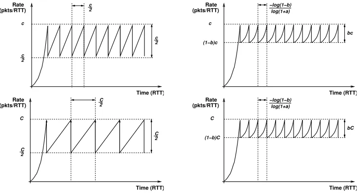
In [106], T. Kelly proposed a new TCP variation called scalable TCP. The basic idea behind STCP is that unlike traditional TCP, whose loss recovery time is proportional to both congestion window size and RTT, the loss recovery time for STCP only depends on RTT. The algorithm of STCP can be generalized as [106]

(28)

Auto Hiperf Default Mbytes

conns 0.00

0.20 0.40 0.60 0.80 1.00 1.20 1.40 1.60 1.80 2.00 2.20 2.40 2.60 2.80 3.00 3.20 3.40 3.60 3.80 4.00

0.00 5.00 10.00 15.00 20.00 25.00 30.00

Figure 2.3: Performance Comparison: Peak usage of memory. Auto: the proposed scheme; Hiperf: Tuning by Hand; Default: Default setting by NetBSD [176].

for each acknowledgement without a loss packet, where 0< a <1. And for each loss occurs

cwnd=cwnd∗(1−b) (2.2)

where 0< b <1. The values ofaand bdepend on implementation and deployment such as legacy traffic, bandwidth and flow rate variance.

(29)

c 2

Rate (pkts/RTT)

c

Time (RTT)

c 2 c

2

C 2

Rate (pkts/RTT)

C

Time (RTT)

Figure 1: Traditional TCP scaling properties.

log(1+a) −log(1−b)

Rate (pkts/RTT)

(1−b)c

Time (RTT)

c

bc

log(1+a) −log(1−b)

Rate (pkts/RTT)

bC

(1−b)C

Time (RTT)

C

Figure 2: Scalable TCP scaling properties.

Figure 2.4: Illustration: Traditional TCP and STCP [106].

High Speed TCP: HSTCP

Floyd, et al. modified TCP as HSTCP in [70, 65, 66]. The objective of HSTCP is to design a congestion control algorithm which obtains a higher sending rate at a given loss rate, while keep the property of TCP-friendliness. The algorithm is also a kind of additional increase and multiplicative decrease (AIMD) with different addition and multiplication.

The objective of HSTCP is to achieve transmission rate of 10 Gbps under realistic packet drop rate environment. Since Floyd has not solidify the design detail, we don’t know how it works so far. It has the following benefits as pointed out in the draft.

• Maintain high transmission rate with reasonable loss rate.

• Reach steady transmission rate pretty fast during slow-start.

• Fast recovery during time-out or congestion loss.

(30)

TCP.

• No router involvement.

Figure 2.5 plots the fairness of HSTCP over regular TCP. As the loss probability increases, the HSTCP tends to have the fair throughput compare to regular TCP.

0 50 100 150 200

1e-10 1e-09 1e-08 1e-07 1e-06 1e-05 0.0001 0.001 0.01 0.1

Highspeed TCP / Regular TCP, Sending Rates

Loss Rate P Relative Fairness (0.11/p^0.32)

Figure 2.5: Fairness of HSTCP over regular TCP [70].

BIC-TCP: BTCP

Moreover, Xu, et al. discussed the binary increase congestion control for high-speed networks in [197]. The authors claims that BIC-TCP achieve the following properties:

• Scalability: HSTCP can obtain 10 Gbps bandwidth with loss rate 1e-7, while BIC-TCP would achieve 10 Gbps with 3.5e-8 loss rate.

• RTT fairness: RTT fairness is defined as the RTT ratio of two competing flows. The order of RTT unfairness is about _√1

RT T.

(31)

• Fairness and convergence: BIC-TCP has better sending rate fairness compared to both HSTCP and STCP. And the convergence of BIC-TCP is faster as well.

Comparison of TCP fairness between BTCP and other TCP variation is depicted in Figure 2.6.

E E E ind are c con We o STCP th we resu m g lin RED (alt

TCP-Friendliness, Drop Tail

0% 10% 20% 30% 40% 50% 60% 70% 80% 90% 100% AI MD BI -T CP HST C P ST CP AI MD BI -T CP HST C P ST CP AI MD BI -T CP HST C P ST CP AI MD BI -T CP HST C P ST CP

Long-lived TCP High-speed

Background Unused

20Mbps 100Mbps 500Mbps 2.5Gbps

Figure 2.6: TCP Fairness [197].

Fast TCP: FTCP

Jin, et al. proposed a Fast TCP, which deploys a delay-based congestion con-trol [100, 99]. In fact, using delay to estimate congestion level was already proposed by [95, 143]. The advantage of delay-based over loss-based method is not significant for low speed networks, while as to high speed networks, delay-based may reach a big improve-ment.

FTCP combines delay-based approach and loss-based method. There are two merits to deploy queueing delay as a congestion measure.

(32)

Moreover, the queueing sampling gives much finer information than loss sampling.

• The dynamics of queues has the right scaling with regard to network capacity, which will help TCP stability as the network capacity scales up.

Flow Level Design:

Table 2.1: Design of Reno, HSTCP, STCP and FAST [100] κi(ωi, Ti) µi(ωi, Ti) pi

Reno _T1

i

1.5

w2

i loss probability

HSTCP 0.16b(ωi)ωi0.8

(2−b(ωi))Ti

0.08

ω1.20 i

loss probability

STCP aωi

Ti

ρ

ω loss probability

FAST γα_i αi

xi queueing delay

where Ti is the round trip time (RTT),ωi is the window size,pi is the congestion

measure,xi=ωi/Ti. Anda, b(ωi), ρ, γ, αi are protocol parameters.

The equilibrium transmission rate, xi, is given by

Table 2.2: Equilibrium Transmission Rate [100] Transmission rate

Reno xi = _T1_i_p0.50αi i

HSTCP x_i = 1

Ti

αi

p0.84 i

STCP xi = _T1_iα_p_ii

FAST xi = α_p_ii

XCP

(33)

introduce a new concept called “decoupling of utilization control from fairness control”. Based on utilization control, XCP reach stability under high speed network with large de-lay, which is believed to be very important to the congestion control protocol. Moreover, XCP has almost all the desirable properties: efficiency, fairness, scalability.

The additional benefits of deploying XCP are the following:

• By deploying XCP, drops due to congestion becomes unusual, because before a drop occurs, an explicit notification is sent back to the sender to reduce the window size.

• XCP is easier to detect attacks and separate the unresponsive flows, which facilitate the network security.

• Gradual deployment: Since XCP is a TCP-friendly congestion control protocol, it can be fairly co-exist with current TCP and its variations.

• XCP enhances network security. For example, XCP can easily detect and isolate the unresponsive sources due to two characteristics: (i) operation with near-zero drops, (ii) explicit feedback.

• QoS: Since XCP decouple of utilization from fairness, it makes Differv service easier to design and implement. In detail, by using efficiency controller, XCP guarantees high utilization and small queues. Therefore, Diffserv is just to apply the aggregate feedback to the individual flows to make them converge to the desired rates.

The design rationales behind XCP are from several aspects.

Extensive simulation results indicate that XCP outperforms TCP over conven-tional AQM (Active Queue Management) such as RED, REM, AVQ, CSFQ (Core Stateless Fair Queue).

TCP-SABUL

(34)

SABUL tries to make a balance between TCP-friendliness and higher transmission rate, which is shown in Figure 2.7.

effectively use the available bandwidth.

Figure 2. This graph shows the performance of three simulated SABUL flows

Figure 2.7: Fairness of TCP SABUL [78].

TCP-Westwood

TCP Westwood [144] is designed to improve TCP performance in both wired and wireless links. Instead of using packet loss, TCP Westwood deploys end-to-end bandwidth as an indicator for network congestion control. Unlike packet loss indicator, end-to-end bandwidth can tell the difference between the packet loss due to network congestion and the packet loss caused by wireless channel fading.

In general, this difference is important for us to reduce the packet loss. Specifically, if the packet loss is the result of network congestion, the TCP should decrease the window size to reduce the work load to the networks. However, if the packet loss is caused by wireless channel fading, the TCP should send more packets to recover the loss ones. We can see that two causes of packet loss may result in the very contrary result. Therefore to apply TCP into wireless link, we should enable TCP to discriminate this difference.

(35)

the overhead to the network design and implementation. In reality, simple approach always gives rise to the robustness.

In detail, TCP Westwood decides a slow start threshold (ssthresh) and a congestion window (Cwnd), which leads to a effective bandwidth corresponding to the congestion. This scheme is called “fast recovery”. Compare with previous TCP version, which simply reduces the Cwnd to half, TCP Westwood can effectively cope with wireless link. Shortly, end-to-end bandwidth estimation is achieved by three steps: (i) ACK-based measurement (ii) Filtering ACK reception rate (iii) detect on the delay and cumulative ACKs. Finally, it is also claimed that TCP Westwood has good throughput and TCP friendly as well, which is displayed in Figure 2.8 and 2.9.

improves its performance but in a less considerable

0 1 2 3 4 5 6 7 8

Bottleneck bandwidth, µ (Mbps)

Average Throughput (Mbps)

Average Throughput, µ=2 Mbps, d=70ms, L=3200 bit/pck, ν=0

TCP Reno TCPW

Figure 2.8: TCPWestwood and TCP-Reno: Throughput vs. bottleneck bandwidth [144].

TCP-Planet

(36)

ies our choice of B=C.

0 10 20 30 40 50 60 70 80 90 1.3

1.4 1.5 1.6 1.7 1.8 1.9 2

Buffer size, B (pck)

Average Throughput (Mbps)

Average Throughput, µ=2 Mbps, d=70ms, L=3200 bit/pck, ν=0

TCP Reno TCPW

Figure 2.9: TCPWestwood and TCP-Reno: Throughput vs. bottleneck buffer size [144].

TCP-Planet also deploys AIMD congestion control algorithm. While AIMD here is tuned to avoid throughput degradation. Further, TCP-Planet modifies the slow start al-gorithm, which is not suitable to inter-planet transmission, to a “Initial State Algorithm”, which would capture the available resource in a fast manner. Moreover, a new conges-tion control algorithm is develop for inter-planet transmission. They introduce “blackout” state into the new protocol to reduce the effect of “blackout”. Finally, a delayed selective acknowledgement (DSACK) is proposed to address the bandwidth asymmetry problem.

Network Proximity

Earth

Planetary Satellite Network Mars

Earth Relay Orbit

Interplanetary Backbone Network (Deep Space Communication Link)

Figure 2.10: Interplanetary Internet [8].

(37)

Immediate

Start Blackout

Rate Decrease

Rate Increase Hold Rate

Φ>φi

Φ<φd

φ <Φ<φd i Φ<φd

Follow−Up

Φ>φi _{φ <Φ<φ}

i d

t=RTT

t= 2*RTT INITIAL STATE

STEADY STATE

Figure 2.11: State Transition Diagram [8].

2.2 TCP over Wireless Networks

With the booming development of wireless networks, TCP over wireless becomes a natural result due to the demand of application. By introducing wireless to TCP, TCP should consider 3 major changes related with loss, because the main objective of TCP is reliable transmission.

1. Congestion loss: Wireless links introduce more traffic to the existing wired backbone. And congestion loss may happen at wireless router, wireless gateway in cellular net-works

2. Handoff loss: This type of loss is unique to TCP over cellular networks. In other environment, either wired or wireless ad-hoc network has no such kind of loss. Since handoff is the procedure that a mobile terminal transfer from one access point to another access point, this process may introduce potential packet loss.

(38)

we briefly describe the 3G cellular network r e phasized,

l is investigated

Τ

) S

Figure 2.12: Three Types of Loss in Cellular Networks.

TCP over Cellular Networks

In [83], Hu, et al. studied the TCP performance in the case of cellular networks. Specifically, the authors proposed a scheme to improve TCP through during handoff. The merit of suggested scheme is that it is kind of fine-tuning to existing TCP, which may reduce the cost in real implementation.

Moreover, a simple Finite State Markov Chain (FSMC) model is suggested to analyze error loss over wireless channel. They use FSMC to study the Rayleigh fading channel. And, coding scheme is also taken into account by FSMC. Finally, they verify their results by NS simulator.

τ

performance (see Fig.4).

» ¼ º «

¬ ª

π π

Figure 2.13: Two State Markov Chain for Loss Channel [83].

(39)

TCP over Ad-hoc, Multi-hop Network

Again, fairness is an important issue for TCP field. Many research has been done to explore the fairness in wired networks. Bottigliengo, et al. studied TCP fairness for 801.11b WLANs in [29].

Traditionally, QoS in wired networks concerns about (i) traffic burstiness (ii) un-predictable nature of the number of users (iii) random access protocols. In addition to these obstacles, WLANs impose more challenges including poor channel qualify, interference from hidden terminals, etc.

802.11b WLAN

WS N WS

N−1

R, D wired link

AP

WS 1

WS 2 WS 3

S

Figure 2.14: Network Scenario for 802.11b WLAN [29].

p

bg_S bg_L

k

1 − k p

LB

SB

gb

p

G

(40)

In order to achieve fairness, the authors propose an LLC-layer algorithm to guaran-teeing fair access to the medium to every user by awarding longer transmission opportunities to short channel failures. Such mechanism can protect short-lived TCP flows.

TCP API for Wireless

In the real world, the implementation of wireless API for TCP is discussed in [20]. In wireless environment, the bandwidth and RTT have a large scale variation, which is unlike the wired link, because the distance between the mobile terminal and the base station is changed over time and the interference received by mobile terminal variation from time to time as well. Fig 1 and 2 in [20] clearly demonstrate such variations.

0 100 200 300 400 500

0 200 400 600 800

time (s)

bandwidth (KB/s)

Figure 2.16: An Example of Bandwidth Variation over time [20].

0 100 200 300 400 500

0 0.05 0.1 0.15 0.2

time (s)

round−trip time (s)

(41)

Atkin, et al., propose an network-aware interface (NAI) for adaptive applications over wireless networks. The API can help the upper level application accurately match the operation to the available bandwidth, i.e, cope with the burst data.

The idea to serve adaptive application is also discussed in [71, 151, 111].

TCP Wireless Header

Another TCP variation happens at TCP header. In [25], Balan, et al. presented a modification to TCP header. This revise enhances TCP to cope with lossy environment. In a short, they deployed two TCP options: (i) TCP header checksum option, (ii) TCP header checksum ACK option, which are given as follows:

Table 2.3: TCP Header Checksum Option [25]. Kind=14 Length=4 1’s complement checksum of

TCP header and pseudo-IP header

Table 2.4: TCP Header Checksum ACK Option [25]. Kind=15 Length=6 32-bit sequence number of

corrupted segment to resend

2.3 Other Related Work of TCP

(42)

TCP Prediction by Sampling

Application sampling is a good way to monitor TCP performance, since it is simple to be deployed. In [76], Goyal, et al. investigate the method to sample the network to predict network parameters such as RTT, loss rate and throughput.

Two sampling methods are proposed in [76].

• (I) Probing: This approach probes the network with end-to-end pings, for instance. Each ping can provide an RTT sample, which can be used to estimate retransmission timeout,T0, along with clock granularity, G.

T0 =srtt+max{G,4×rttvar}

wheresrtt is smoothed RTT, and rttvar is the standard deviation of RTT samples. The pros of probing is that they provide the information of complete networks. There-fore, by probing, we can estimate the end-to-end packet loss probabilities and round-trip times. The cons of probing are that

1. Probing packets do not work the same as the actual TCP flows.

2. Packets loss by probing maybe chang significantly with different number of pack-ets in one round probe, the inter-probe delay, the frequency of probing, and the probing packet size.

3. The convergence of packet loss probabilities is slow.

4. Due to IP routing policy, probing packets may not follow the same path as the packets in real transmission.

(43)

One thing to avoid by such sampling approach is over-sampling, which may incur unnecessary overhead to the networks. In general, session level and network level informa-tion is used to predict the throughput of TCP flows. The session level parameters consist of packet size, window size, retransmission timer and ACK. The network level parameters include RTT and loss rate.

TCP Prediction by Passive Measurements

The idea of passive measurement is new and interesting [96]. Instead of measuring the TCP connection at end point, the authors keep track of TCP parameters in the middle way of an end-to-end path.

The benefits of estimating RTT and CWND are that

1. They help us know the factors affecting TCP throughput.

2. They can be used to probe nonconforming TCP senders, and to distinguish different type of TCP implementations in reality.

3. They also can provide information on revealing the enhanced capability of new ver-sion TCP. For example, how often TCP Reno’s fast recovery is actually deployed in practice.

Observations:

1. The bottleneck for the throughput is in most cases that the send do not have enough data to send, rather than the network’s capability.

2. It shows that up to now, TCP/newreno is the dominant implementation at end host. 3. Another important observation is that in general, the RTTs of one connection don’t suffer large variation during the transmission. This is a good news for end-to-end multimedia transmission. That is, the bandwidth will not great degradation.

RTT estimation is described in [96]:

(44)

Potential estimation error:

1. Under-estimate of cwnd: When duplicate ACKs loss happens, their method may indicate that the sender will launch a fast retransmission, which may cause cwnd and ssthresh decreased accordingly. Therefore, the proposed method will count ssthresh reduction twice. However, due to loss ACKs, the actual sender only reduce ssthresh once.

2. Over-estimate of cwnd: There are two cases, which may cause a over estimation for their measurement. Case I: The acknowledgements lost after they pass the measure-ment point. Case II: All of the data belongs to the current window lost before they reach the measurement point.

TCP Start-Up Prediction

In general, TCP start-up performance refers to the delay of three-way handshake for connection establishment and slow start. Cardwell, et al. proposed a model for TCP latency in [37].

There are three major assumptions for their model:

1. The sender is TCP/Reno family. However, the model can be applied to TCP/Newreon, SACK or FACK.

2. The random variable, r.v. for he loss in one round is I.I.D (Independent Identically distributed).

3. The connection could be few packet loss and be dominated by TCP connection setup and initial slow start.

Connection Setup Latency:

The procedure of three way handshake is illustrated in Figure 2.18. The predicted handshake time is given by

E[Dh] =RT T+Ts×(1₁−pr

2pr +

(45)

SYN x

SYN y, ACK x+1

ACK y+1

Active Opener

Passive Opener

iFailures

jFailures

Connection Effectively Established

Figure 2.18: Illustration of TCP Connection Establish [37].

where Ts is the SYN timeout, pf is the forwarding packet loss rate and pr is the reverse

packet loss rate.

Slow Start Latency:

The predicted slow start latency is given by

E[Tss] =

 



RT T ×[log_r(Wmax

ω1 ) + 1 +

1

Wmax(E[dss]−

γWmax−ω1

γ−1 )] if E[Wss]> Wmax RT T ×log_r(E[dss](γ−1)

ω1 + 1) if E[Wss]≤Wmax

whereE[dss] is the number of data segment to be sent in the slow start phase given by

E[dss] = (1−(1−p)

d₎₍₁₋_p)

p + 1

wherep is the data segment loss rate.

And E[Wss] is the expected window size after slow start given by

E[Wss] = E[dss](γ_γ −1)+ω_γ1

(46)

TCP Latency and Throughput Prediction

Prediction of TCP performance has been extensively studied in many literatures [110, 154, 127, 145, 93, 149, 152]. In [110], Sikdar, et al. analyzed latency and steady state throughput of the major TCP versions: Tahoe, Reno, SACK.

The assumption they use are the following:

1. Only the delays of TCP performance is considered and other delays such as buffer delay is not taken into account.

2. The sender always has data to transmit, i.e., the congestion window is fulfilled always. 3. The window size of the receiver is not changed over time.

4. The acknowledgement by the receiver is the same as RFC 2581. 5. Nagle’s algorithm and silly window avoidance is ignored.

6. TCP latency is presented in terms of RTT.

Generally speaking, TCP Tahoe deploys the slow start, congestion avoidance and fast recovery algorithm to TCP [91]. TCP Reno adds fast-retransmission to TCP. And TCP Sack improves Reno on recovery for multi-loss in one timeout.

TCP Latency:

The predicted transmission time is generalized as follows [110]

Ttransf er(N) =tsetup+tdack+ (1−p)Ntnl(N) +p(1−p)N−1E{tsl(N)}+tml(N)

where Ttransf er(N) is the transmission time for N packets, tsetup is the TCP setup time.

tdack is the delayed acknowledge time. tnl is the transmission time forN packets. tsl is the

time for N packets with a single loss indication. And tml is the transmission time for N

packets withM loss indication.

For example, in the case of TCP Tahoe, tsetup, tnl(N), tsl(N), tml(N) are given

(47)

•

tsetup =RT T + 2Ts(

1−p 1−2p −1)

•

t_nl(N) =

 



d2 log₂(₂2√N+4+3√2

2+3(2)5/8)eRT T if N ≤Nexp h

nwm+dN_W−_maxNexpe

i

RT T o.w.

•

tsl(N) =

 



[t_nl(i) +r(n) + 1 +t_lin(a, b)]RT T if nrnd1

i ≥3

£

t_nl(i) +r(n) +t_lin(a, b) +I(nrnd1

i >0) +E[T O]

¤

RT T o.w.

•

tml(N) =E{tsl(m−1)}+ (M−2)E{tM loss(Dave)}

TCP Throughput:

The throughput can be represented by [110]

T hp= dM SS tss(p) =

M SS tss(p)p

wheret_ss(p) is the expected time to transmit dpackets given by

tss(p) = _c 2 wm(cwm+ 1)

cwm X h=1 h X j=1

tM loss(d)

wherecwm is defined by

cwm= min{



−1 +

q 1+16 p 2   +

, Wmax}

Even though the close form of the throughput is different from that in [154], the results match with each other. Figure 2.19 compares the throughput of three schemes.

2.4 Active Queue Management: AQM

(48)

(a) (b) (c) Fig. 6. Transfer times and steady-state throughput for Tahoe, Reno, and SACK for (a), (b) correlated and (c) independent losses.

Figure 2.19: Throughput Comparison of Tahoe, Reno and Sack for (a), (b) correlated and (c) independent losses [154].

may yield better performance. In general, there are three representative AQM schemes: Random Early Detection (RED), Random Exponential Marking (REM) and Adaptive Vir-tual Queue (AVQ). Based on RED, there are some derivatives such as BLUE, GREEN and PI.

RED

Sally Floyd and V. Jacobson revolutionarily propose Random Early Detection (RED see [69]) routers and Explicit Congestion Notification (ECN see [62]) to help TCP end-to-end congestion avoidance in packet-switched networks.

(49)

certain probability, where the dropping or marking probability is determined by a function of the average queue size. By marking a packet, the router set a the ECN bit in the TCP header to notify the receiver that there is congestion in the middle of the network. After receiving such an notification, the TCP sender will reduce the window size, i.e., decrease the transmission rate, which may mitigate the workload to the network. With the help of the third party, TCP congestion control may outperform TCP stand alone.

Moreover, routers with RED keep the average queue size low while allowing oc-casional bursts of packets in the queue. During congestion, the probability that the router notifies a particular connection to reduce its window is roughly proportional to that connec-tions share of the bandwidth through the router. RED routers are designed to cooperate with TCP. Further, as the authors pointed out that RED router has no bias against bursty traffic and avoids the global synchronization of many connections decreasing their window at the same time. The performance of RED plus ECN is depicted in Figure 2.20.

From 1993, RED experienced a rapid development such as FRED, SRED, BLUE etc. Most of research work can be categorized into the following groups by Sally Floyd [61], which gives us a very good overview on AQM (cf. many thanks to Sally Floyd).

• Enhance RED queue management [30, 67].

• Evaluation of RED [49, 146, 39, 64, 204, 34].

• Modification of RED and other AQM [18, 22, 23, 55, 56, 57, 34, 35, 92, 115, 116, 153, 169, 170, 205].

• RED with Drop Preference [41, 26].

• RED with per Flow Information [131, 16, 4, 142, 182].

(50)

Drop Tail, TCP clock = 100 msec Switch Buffer Size (in kB)

Bulk-Data Throughput

0 50 100 150 200

0.0

0.2

0.4

0.6

0.8

1.0 x===ooo_o_o+=xxxx=++++ x==++++oo=ooo=+=xxxx x====ooooo=+x++++xxx ====xo+++++++++oxxxxooo=

+ : byte-based DT, 8 kB windows x : packet-based DT, 8 kB windows

o : byte-based DT, 64 kB windows = : packet-based DT, 64 kB windows

RED without ECN, TCP clock = 100 msec Switch Buffer Size (in kB)

0 50 100 150 200

0.0

0.2

0.4

0.6

0.8

1.0 +++++ +++++ +++++ +++++

x x x x

x xxxxx xxxxx xxxxx

o o o o o o o o o o _ooooo

o o o o o = = = = = = = = = = ===== =====

RED with ECN, TCP clock = 100 msec Switch Buffer Size (in kB)

0 50 100 150 200

0.0

0.2

0.4

0.6

0.8

1.0 +++++xxxxx xxxxx+++++ +++++xxxxx +++++xxxxx

o o o o

o ooooo ooooo ooooo =

= = =

= ===== ===== =====

Smallest Bulk-Data Throughput

0 50 100 150 200

0.0

0.05

0.10

0.15

0.20 +++++xxxxx xxxxx+++++ +xx+xxx+++ xxxx+++++++++x

o o o o o o o o o o o o o o o o o o o o = = = = = = = = = = = = = = = = = = = =

0 50 100 150 200

0.0 0.05 0.10 0.15 0.20 + + + + + + + + + + +++++ ++ + + + x x x x x x x x x x x x x x x xxxxx

o o o o o o o o o o o o o o o o o o o o = = = = = = = = = = = = = = = = = = = =

0 50 100 150 200

0.0

0.05

0.10

0.15

0.20 +++++xxxxx xxxxx+++++ +++++xxxxx +++++xxxxx

o o o o

o ooooo ooooo _ooooo = = = = = ===== ₌==== = = = = =

Highest Telnet Delay (in Seconds)

0 50 100 150 200

0 1 2 3 4 + + + + + +++++ +++++ +++++++++ x x x x

x xxxxx xxxxx xxxxx o o o o o o o o o o o o o o o o o o o o = = = = = = = = = = = = = = = = = = = =

0 50 100 150 200

0 1 2 3 4 + + + + + +++++ +++++ +++++ x x x x x x x x x x x x x x x x x x x x o o o o o o o o o o o o o o o ooooo = = = = = = = = = = = = = = = = = = = =

0 50 100 150 200

0.0 1.0 2.0 3.0 + + + + + +++++ +++++ +++++ x x x x

x xxxxx xxxxx xxxxx o

o o o

= = =

= ===== ===== =====

Average Telnet Delay (in Seconds)

0 50 100 150 200

0.0 0.05 0.10 0.15 0.20 + + + + + +++++ +++++ +++++++++ x x x x

0 50 100 150 200

0.0 0.05 0.10 0.15 0.20 + + + + + +++++ +++++ +++++ x x x x x x x x x x x x x x x x x x x x o o o o o o o o o o o o o o o ooooo = = = = = ==== = = = = = = = = = = =

0 50 100 150 200

0.0 0.05 0.10 0.15 0.20 + + + + + +++++ +++++ +++++ x x x x

o o o

= = =

= ===== ===== =====

Fraction of Packets with High Delay

0 50 100 150 200

0.0 0.05 0.10 0.15 0.20 + + + + + +++++ +++++ +++++++++ x x x x

0 50 100 150 200

0.0 0.05 0.10 0.15 0.20 + + + + + +++++ +++++ +++++ x x x x

x xxxxx xxxxx x x x x x o o o o o o o o o

o _o_o_o_o_o _o_o_o_o_o = = = = = = = = = = = = = = = = = = = =

0 50 100 150 200

0.0 0.05 0.10 0.15 0.20 + + + + + +++++ +++++ +++++ x x x x

o o o

= = =

= ===== ===== =====

(51)

REM

Steven Low, et al. propose another AQM: Random Exponential Marking (REM) in [18, 135, 19, 155, 198, 5, 133, 199, 35, 156] to overcome the shortcoming of RED such as poor utilization and stability.

Two features which make REM different from REM are that (i) REM deploy a different marking function. Compared to RED, which uses uniform distributed marking function, REM uses exponential distributed marking function. The comparison is illustrated in Figure 2.21.

Figure 2.21: REM Marking Function compared to RED [18].

(ii) The measurement of congestion of REM is different from that of RED. RED uses average queue size as the congestion measure, while REM defines a price function as the measurement of congestion, which is given by [18]

pl(t+ 1) = [pl(t) +γ(αl(bl(t)−b∗l) +xl(t)−cl(t))]+

where p_l(t) is the price for queue l in period t,γ >0 and α >0 are small constants, b_l(t) is the aggregate buffer size at queue l in period t, b∗_l is target queue length, xl(t) is the

aggregate input rate to queue l in period t, and cl(t) is the available bandwidth to queue

l at period t. The term of xl(t)−cl(t) gives the rate difference and the term of bl(t)−b∗_l

Performance Analysis of TCP over Wired and Wireless Network

Contents

List of Figures

List of Tables

Chapter 1

Introduction

1.1

Motivation

1.2

Contribution

1.3

Outline

Chapter 2

Background of TCP

2.1

TCP over Wired Networks

2.2

TCP over Wireless Networks

Τ

τ

τ

2.3

Other Related Work of TCP

2.4

Active Queue Management: AQM