Scholarship@Western
Scholarship@Western
Electronic Thesis and Dissertation Repository
10-2-2012 12:00 AM
A Study for Detection of Drift in Sensor Measurements
A Study for Detection of Drift in Sensor Measurements
Sungwhan Cho
The University of Western Ontario
Supervisor Jin Jiang
The University of Western Ontario
Graduate Program in Electrical and Computer Engineering
A thesis submitted in partial fulfillment of the requirements for the degree in Doctor of Philosophy
© Sungwhan Cho 2012
Follow this and additional works at: https://ir.lib.uwo.ca/etd Part of the Signal Processing Commons
Recommended Citation Recommended Citation
Cho, Sungwhan, "A Study for Detection of Drift in Sensor Measurements" (2012). Electronic Thesis and Dissertation Repository. 903.
https://ir.lib.uwo.ca/etd/903
This Dissertation/Thesis is brought to you for free and open access by Scholarship@Western. It has been accepted for inclusion in Electronic Thesis and Dissertation Repository by an authorized administrator of
(Spine title: A Study for Detection of Drift in Sensor Measurements)
(Thesis format: Monograph)
by
Sungwhan Cho
Graduate Program in Electrical and Computer Engineering
A thesis submitted in partial fulfillment
of the requirements for the degree of
Doctor of Philosophy
The School of Graduate and Postdoctoral Studies
The University of Western Ontario
London, Ontario, Canada
c
School of Graduate and Postdoctoral Studies
CERTIFICATE OF EXAMINATION
Supervisor Examiners
Dr. Jin Jiang Dr. Vijay Parsa
Dr. James C. Lacefield
Dr. Michael D. Naish
Dr. Steven Ding
The thesis by
Sungwhan Cho
entitled:
A Study for Detection of Drift in Sensor Measurements
is accepted in partial fulfillment of the
requirements for the degree of
Doctor of Philosophy
Date Chair of the Thesis Examination Board
This study aims to develop methods for detection of drift in sensor measurements. The study
consists of three major components; 1) residual generation, 2) statistical change detection, and
3) model building.
To identify the statistical properties of the residuals and to utilize them for detection of the
drift, a new method for estimation of the drift rate is proposed. The method formulates an
augmented system matrix model and processes the model using a Kalman filter. An analytical
method for estimation of the drift rate is also derived. A Hamiltonian approach is used for
evaluation of the steady state covariance of the residuals. The steady state covariance and the
estimated drift rate enable the existence of the drift in the measurements to be determined in a
statistical way using the change detection algorithms.
The statistical change detection algorithms process the residuals to determine the drift
statistically. In the study, performance of the major algorithms, including the Exponentially
Weighted Moving average (EWMA), Cumulative Sum (CUSUM) control chart, and
Gener-alized Likelihood Ratio Test (GRLT), are investigated. A new method for detection of the
change, named the “Standardized Sum of the Innovation Test (SSIT),” is also proposed. The
statistical properties of the decision function of the SSIT are derived to set the decision
thresh-old statistically. A method for estimation of the mean delay of the SSIT is also derived. The
mean delay of the SSIT is shown in a demonstration and is the shortest of the change detection
algorithms.
For demonstration purposes, mathematical models of a pressurizer in a CANada Deuterium
Uranium (CANDUR) nuclear power plant are developed. The mathematical models in the form
of nonlinear differential equations are verified by comparing the simulation results with those
of the industry standard code known as “CATHENA” (Canadian Algorithm for Thermal
pressurizer model for detection and estimation of pressure sensor drift. The results
convinc-ingly demonstrate the effectiveness of the proposed algorithms in the detection of the drift.
Keywords: Statistical Change Detection, Sensor Fault Detection, Sensor Drift,
Standard-ized Sum of the Innovation Test, CUSUM, SPRT, GLRT, Pressurizer,CANDU Reactors.
To my son and daughter, Seyong and Serin.
I am indebted to many individuals who have helped me complete this thesis. These individuals
have not only made important contributions to the preparation and completion of the thesis but
also inspired me to enjoy the process of learning along the way.
I first wish to express my sincere gratitude to Dr. Jin Jiang, my supervisor at the University
of Western Ontario. Without his consistent encouragement and guidance, it would not have
been possible to complete this thesis. I will never forget his pedagogic feedback and
discus-sions which kept me motivated.
Next, I wish to thank all the members of the Nuclear Control and Instrumentation group at
Western for their kind friendship and giving me the opportunity to broaden my knowledge and
interests into different areas of study.
I also wish to thank the engineers at the Wolsong Nuclear Power Plants of the Korea
Hy-dro and Nuclear Power Corporation (KHNP) and the researchers at the Korea Electric Power
Research Institute (KEPRI) for providing me with detailed and practical information regarding
the industrial practices and standards upon which this thesis is based so that I could deliver
better solutions.
Finally, I owe a special debt of gratitude to my wife, Kyunghee, for her love and patience.
She provided the invaluable support and consistent companionship that made the whole period
of the Ph.D. study the most pleasant adventure.
Certificate of Examination ii
Abstract iii
Dedication v
Acknowledgements vi
List of Tables xiii
List of Figures xiv
List of Abbreviations and Nomenclature xvii
1 Introduction 1
1.1 Motivations . . . 1
1.2 Problem Statements . . . 3
1.3 Objectives of the Study . . . 4
1.4 Scope and Contributions of the Study . . . 5
1.4.1 Fundamental Study . . . 6
1.4.1.1 Residual Generation . . . 6
1.4.1.2 Statistical Change Detection . . . 7
1.4.2 Application Study . . . 8
1.4.3 Contributions . . . 8
1.5 Organization of the Thesis . . . 10
2 Residual Generation for Detection of Drift 12 2.1 Approaches to Residual Generation . . . 15
2.2 Change in the Expectation of the Innovation Sequence . . . 17
2.2.1 Linear Discrete Time System with Noise . . . 18
2.2.2 Linear Discrete Time Kalman Filter . . . 18
2.2.3 Innovation Sequence in the Presence of Drift in Measurements . . . 21
2.2.4 A PrioriEstimation Error in the Presence of Drift . . . 22
2.2.5 Expectation of the Innovation Sequence in the Presence of Drift . . . . 22
2.3 Estimation of the Drift Rate by a Kalman Filter . . . 24
2.3.1 Augmentation of the Drift Rate into System Model . . . 24
2.3.2 Expectation of the Innovations with the Augmented Kalman Filter . . . 26
2.3.3 A PrioriEstimation Error after the Augmentation . . . 27
2.3.4 Calculation of the Expectation of the Innovation Sequence . . . 28
2.4 Steady State Covariance of the Innovations . . . 29
2.4.1 Discrete Algebraic Riccati Equation . . . 30
2.4.2 Hamiltonian Approach for a Solution to the DARE . . . 31
2.4.2.1 Hamiltonian Matrix . . . 31
2.4.2.2 Symplectic Matrix . . . 32
2.4.2.3 A Solution to the DARE . . . 33
2.4.3 A Solution to the Steady State Covariance of the Innovations . . . 33
3 Statistical Change Detection Algorithms 36
3.1 Change Detection Algorithms in the Literature . . . 37
3.1.1 Exponentially Weighted Moving Average Control Charts . . . 39
3.1.1.1 Decision Function of the EWMA Control Chart . . . 39
3.1.1.2 Average Run Length Function of the EWMA Control Chart . 40 3.1.2 CUSUM Control Charts . . . 41
3.1.2.1 Decision Function of the CUSUM Control Chart . . . 41
3.1.2.2 ARL Function of the CUSUM Control Chart . . . 42
3.1.3 Generalized Likelihood Ratio Test . . . 42
3.1.3.1 Decision Function of the GLRT . . . 42
3.1.3.2 ARL Function of the GLRT . . . 43
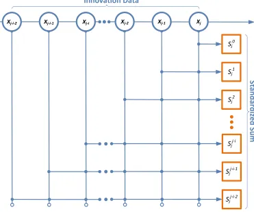
3.2 Standardized Sum of the Innovation Test . . . 44
3.2.1 Decision Function and Stopping Rule of the SSIT . . . 45
3.2.2 Properties of the SSIT . . . 48
3.2.2.1 Decision Function of the SSIT under a Changed Condition . . 48
3.2.2.2 Decision Function of the SSIT under the Mixture of the Changed and Unchanged Conditions . . . 50
3.3 Comparison of the SSIT, EWMA, and CUSUM . . . 56
3.3.1 Mean Delay of the SSIT . . . 56
3.3.2 Mean Delay of the EWMA . . . 57
3.3.3 Mean Delay of the CUSUM . . . 60
3.4 Summary . . . 61
4.1 Analytic Models of the Pressurizer . . . 63
4.1.1 Design Features of the Primary Heat Transport System . . . 63
4.1.1.1 Pressure and Inventory . . . 64
4.1.1.2 Control of the Pressure and Inventory of PHT . . . 65
4.1.1.3 Changes in Pressurizer Process Variables to Disturbances and Failures . . . 66
4.1.2 Nonlinear Differential Equation Representations of a Pressurizer . . . . 67
4.1.2.1 Change in Pressure . . . 74
4.1.2.2 Change in Enthalpy . . . 75
4.1.2.3 Change in Liquid Volume . . . 77
4.2 Water Property Evaluation . . . 78
4.2.1 Liquid Region (Region 1) . . . 79
4.2.1.1 νL(P,T) . . . 80
4.2.1.2 ∂νL(P,T)/∂P . . . 81
4.2.1.3 ∂νL(P,T)/∂T . . . 82
4.2.1.4 TL(P,h) . . . 83
4.2.1.5 ∂TL(P,h)/∂h . . . 83
4.2.1.6 ∂νL(P,h)/∂h . . . 84
4.2.2 Vapor Region (Region 2) . . . 85
4.2.2.1 νV(P,T) . . . 85
4.2.2.2 ∂νV(P,T)/∂T . . . 87
4.2.2.3 ∂νV(P,T)/∂P . . . 87
4.2.2.4 Tv(P,h) . . . 88
4.2.2.6 Tv(P,h),∂TV(P,h)/∂hfor sub-region (2b) . . . 90
4.2.2.7 Tv(P,h),∂TV(P,h)/∂hfor sub-region (2c) . . . 90
4.2.2.8 ∂νV(P,h)/∂h . . . 91
4.3 Verification of the Model . . . 92
4.3.1 Simulations of the Pressurizer Models . . . 92
4.3.1.1 Discrete Time State Space Representation of the Pressurizer . 92 4.3.1.2 Linearization Error . . . 95
4.3.2 Comparison between the Responses from the Developed Model and CATHENA Simulation . . . 97
4.3.2.1 Response to Surge . . . 98
4.3.2.2 Response to Heater Operation . . . 104
4.4 Summary . . . 106
5 Demonstration of Drift Detection Using the Pressurizer Models 108 5.1 Discrete Kalman Filter for the Pressurizer . . . 109
5.2 Statistical Properties of the Innovations of the Pressurizer Model . . . 112
5.2.1 Drift Effect on the mean of the Innovation Sequence . . . 112
5.2.2 Calculation of the steady state covariance . . . 116
5.2.3 Comparison of the Mean and the Variance of the Innovations . . . 119
5.3 Simulations of the Change Detection Algorithms . . . 121
5.3.1 Behavior of the Decision Functions . . . 121
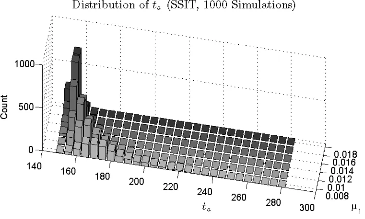
5.3.2 Distribution of the Detection Time . . . 125
5.4 Summary . . . 139
6.1 Summary . . . 140
6.2 Conclusions . . . 143
6.3 Suggestions for Future Work . . . 145
6.3.1 Analytic Solution to the Standard Deviation of the Decision Function of the SSIT . . . 145
6.3.2 Robustness of the SSIT . . . 145
6.3.3 Recursive Version of the SSIT . . . 145
6.3.4 Pressurizer Models under Different Operating Conditions . . . 146
6.3.5 Water Properties for Different Regions . . . 146
Bibliography 147
Curriculum Vitae 152
3.1 Parameter values for comparison of the algorithms . . . 56
3.2 Comparison of the mean delay by calculations (Unit: Samples) . . . 59
4.1 Level deviations after 40sec. . . 99
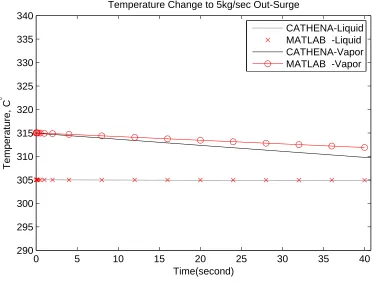
4.2 Temperature deviations(C◦) after 40sec. . . 102
4.3 Pressure deviations(MPa) after 40sec. . . 103
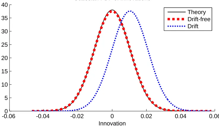
5.1 Comparison of the mean and the variance of the innovations of the pressure . . 120
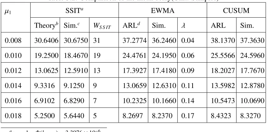
5.2 Comparison of the mean delay(Unit: Samples) . . . 125
5.3 Maximum and standard deviation of the detection time(Unit: Samples) . . . 131
List of Figures
1.1 Organization of the Thesis . . . 11
3.1 Generation of the backward standardized sum . . . 46
3.2 The change in the expectation of the test statistics of the SSIT . . . 51
3.3 Lower bound of the mean delay by the SSIT . . . 57
3.4 Optimalλfor the EWMA . . . 59
3.5 Comparison of the mean delay . . . 60
4.1 Primary heat transport system of a CANDUR plant . . . 64
4.2 Illustrative diagram of a pressurizer . . . 69
4.3 Input output relations of the pressurizer . . . 79
4.4 Simulation results of the pressurizer based on the nonlinear model . . . 96
4.5 Comparison between the simulation results based on the nonlinear and the lin-ear discrete pressurizer model . . . 97
4.6 Level change subject to surge events . . . 99
4.7 Temperature response subject to a surge event(5kg/secout-surge) . . . 100
4.8 Temperature response subject to surge events(8kg/secout-surge, and 10kg/sec in-surge) . . . 101
4.9 Pressure change to surge events . . . 103
4.10 Level and pressure change subject to heater operation . . . 105
5.1 Noises and simulated drift added to the pressurizer model . . . 112
5.2 Pressure(A posterioriKalman filter estimation) . . . 113
5.3 Drift estimations and innovations . . . 114
5.4 Comparison of the innovations under the Kalman filter structures . . . 115
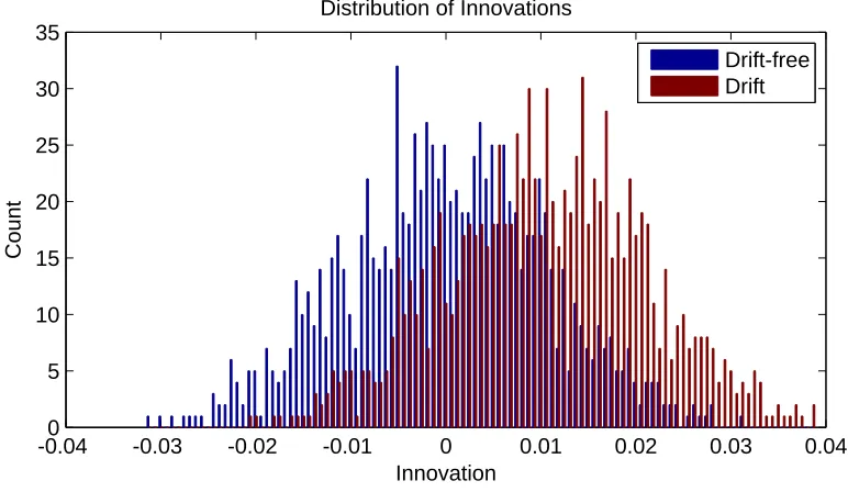
5.5 Time trajectories ofa prioriestimation error and the variance of the innovations 118 5.6 Histograms of the innovation sequence . . . 119
5.7 Probability density functions of the innovation sequence . . . 120
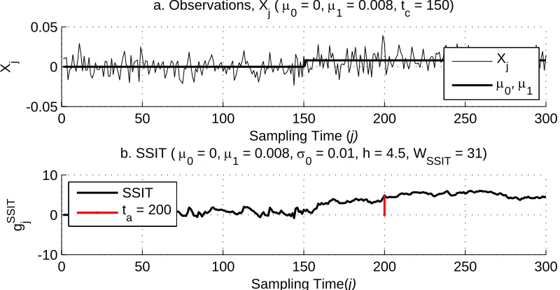
5.8 Observations and change detection by the SSIT (µ1 =0.008) . . . 122
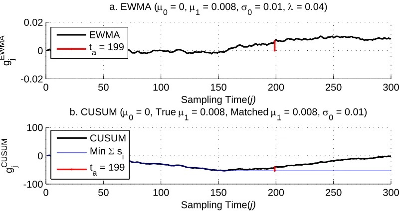
5.9 Change detection by the EWMA, CUSUM (µ1= 0.008) . . . 123
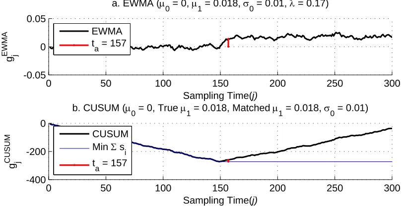
5.10 Observations and change detection by the SSIT (µ1 =0.018) . . . 124
5.11 Change detection by the EWMA, CUSUM (µ1= 0.018) . . . 124
5.12 Distribution of the detection time (SSIT) . . . 126
5.13 Mean delay (SSIT) . . . 127
5.14 Distribution of the detection time (EWMA) . . . 128
5.15 Mean delay (EWMA) . . . 128
5.16 Distribution of the detection time (CUSUM) . . . 129
5.17 Mean delay (CUSUM) . . . 129
5.18 Distribution of the detection time (µ1= 0.008) . . . 130
5.19 Comparison of the distribution of the detection time (µ1= 0.008) . . . 131
5.20 Mean and standard deviation of the detection delay (by simulations) . . . 133
5.21 Maximum detection time(by simulations) . . . 133
5.22 Distribution of the detection time (µ1= 0.01) . . . 134
5.23 Comparison of the distribution of the detection time (µ1= 0.01) . . . 134
5.25 Comparison of the distribution of the detection time (µ1= 0.012) . . . 135
5.26 Distribution of the detection time (µ1= 0.014) . . . 136
5.27 Comparison of the distribution of the detection time (µ1= 0.014) . . . 136
5.28 Distribution of the detection time (µ1= 0.016) . . . 137
5.29 Comparison of the distribution of the detection time (µ1= 0.016) . . . 137
5.30 Distribution of the detection time (µ1= 0.018) . . . 138
5.31 Comparison of the distribution of the detection time (µ1= 0.018) . . . 138
Abbreviations
ACR Advanced CANDUR Reactor
ARL Average Run Length
ASN Average Sample Numbers
CANDUR
CANada Deuterium Uranium
CATHENA Canadian Algorithm for Thermal Hydraulic Network Analysis
CUSUM CUmulative SUM
DARE Discrete Algebraic Riccati Equation
DCC X, Y Digital Control Computer X, Y
EWMA Exponentially Weighted Moving Average
FDI Fault Detection and Isolation
FSAR Final Safety Analysis Report
GRLT Generalized Likelihood Ratio Test
LOCA Loss of Coolant Accident
LOFT Loss of Fluid Test
MATLABR
MATrix LABoratory
NPP Nuclear Power Plant
NPSH Net Positive Suction Head
PDF Probability Density Function
PHT Primary Heat Transport
PIC Pressure and Inventory Control
RIH Reactor Inlet Header
ROH Reactor Outlet Header
SLAE Systems of Linear Algebraic Equations
SPRT Sequential Probability Ratio Test
SRP Standard Review Plan
SSIT Standardized Sum of the Innovation Test
WGN White Gaussian Noise
Nomenclature
Fk state transition matrix
Gk control input matrix
gi decision function
gi decision function of EWMA
g(P,T) specific Gibbs free energy as a function of pressure and temperature
Hk measurement model
hS S IT SSIT threshold
hE EWMA threshold
hC CUSUM threshold
H Hamiltonian matrix
hcs specific enthalpy of condensing spray (kJ/kg)
hL specific enthalpy of liquid phase (kJ/kg)
hsp specific enthalpy of spray (kJ/kg)
hsu specific enthalpy of surge (kJ/kg)
hV specific enthalpy of vapor phase (kJ/kg)
IS S steady state value of the covariance of the innovations
J skew symmetric matrix
Jx Jacobian Matrix of x
Ju Jacobian Matrixu
Kk Kalman filter gain
K(θ, θ0) Kullback information between the probability density fθ and fθ0
LL liquid level (m)
L(z) ARL function when the decision function starts fromz
M symplectic matrix
mcs mass of steam condensing into the pressurizer (kg)
mL mass of water in the liquid region (kg)
msp mass of spray injected into the pressurizer (kg)
msu mass of water entering the surge line and mixing with liquid (kg)
mV mass of vapor in the vapor region (kg)
N(µ, σ2) Gaussian distribution with meanµand varianceσ2
P pressurizer pressure (MPa)
P−
k a prioricovariance of the state estimation error
P+k a posterioricovariance of the state estimation error
Pµ(X) probability density function X
Qh energy added by the heater (kJ)
Qi exponentially weighted moving average
Qk process noise covariance matrix
Rk measurement noise covariance matrix
si log likelihood ratio at timei
Si sum of log likelihood ratio at timei
T temperature
TL liquid temperature
TV vapor temperature
TCUS U M detection time by CUSUM
TEW MA detection time by EWMA
TGLRT detection time by GLRT
T r(·) trace of matrix (·)
ta detection time
tc change time
UL internal energy of liquid phase (kJ)
UV internal energy of vapor phase (kJ)
V pressurizer volume (m3)
VL pressurizer liquid region volume (m3/kg)
VV pressurizer vapor region volume (m3/kg)
vk measurement noise
wk process noise
Xi measurement taken at each time (i=1,2, . . .)
x0 initial process state
xk process state
x−k a prioristate estimate
x+k a posterioristate estimate
ˆ
x+0 initial state estimate
yk measurement
yD
k measurement with drift
α drift rate vector
α0 type I error probability
β0 type II error probability
µ mean of the measurement sequence
µ0 mean of the measurement sequence before change
µ1 mean of the measurement sequence after change
νV specific volume of vapor (m3/kg)
νL specific volume of liquid (m3/kg)
¯
τd mean delay of the detection
Φ(x) Gaussian cumulative distribution function of x Ψ eigenvector matrix ofM
ψk,i state transition matrix
Chapter 1
Introduction
1.1
Motivations
To achieve high level safety and performance, the process parameters (such as voltage,
cur-rent, pressure, temperature, level, etc.) of an industry plant are measured and controlled by
instrument systems. Maintaining a high level of accuracy in the instrument systems is a
criti-cally important task for the safety and performance requirements; however, the measurements
made by the instrument systems have some level of intrinsic uncertainty caused by a variety
of inaccuracies such as; measurement inaccuracy, sensor drift, sensor calibration inaccuracy,
rack calibration inaccuracy, rack drift, etc.[1]. The measurements of the process parameters
can also contain electrical noise due to electromagnetic interference and temporal fluctuations
from vibrations or disturbances.
If the measurement output shows a bias which increases slowly in time independent of
the measured property, this is defined as measurement drift [2]. The measurement drift in the
displays or chart recorders or reach a level to trigger the system alarms. As a result, the
ex-istence of the drift in the measurement is difficult to detect and distinguish from the intrinsic
errors and noise in the measurements. If a drift is not detected promptly enough, not only will
the product of the plant not meet the specified quality but the safety margin of the systems can
also be reduced by the measurement drift. The risk of harming the plant, the public, and the
environment can be increased and a catastrophic accident may occur from the reduced safety
margin.
An example of a significant result from the measurement drift can be found in the cases
of the feed water flow rate measurements of nuclear power plants[3]. The measurement drift
caused by the venturi meter fouling resulted in power derating of the nuclear power plant.
The report shows the amount of derating on average was between 1 and 2% of full power. A
derating of 2% in an 800-MW(electric) unit will cost the utility about $20000/day given that
the cost of electricity is $0.05/kWh [4].
In nuclear power plants, the codes and standards [5][6][7][8] enforced by governing
au-thorities require the sensors measuring the process parameters of the systems containing a high
density of energy or hazardous materials to be tested and calibrated regularly to reduce the risk
caused by the measurement drift. The codes and standards often require hardware redundancies
to reduce the risk from the uncertainties from the instruments as well.
The components of the instrument system outside the physical system boundary can be
tested and calibrated on-line while the plant is in 100% full power operation but the sensor
calibrations are performed while the plant is undergoing a scheduled overhaul. Based on the
uncertainties specified by the manufacturers of the sensors, a certain amount of safety margin
is imposed by the codes and standards when designing the set-point for alarms or shutdown of
In short, hardware redundancies, periodic calibrations, and safety margins are the major
requirements imposed on the industry to cope with the uncertainties from the sensor drift.
However, in addition to the current requirements for the industry, there have been rigorous
studies proposing algorithms for detection of the faults in the Fault Detection and Isolation
(FDI) literatures [9][10][2][11]. The change detection algorithms [12][13] can also be used in
connection with the FDI algorithms. Some algorithms focus on detection of the fault while
others focus on the location of the fault. Investigations into the algorithms presented in the
literature which can be practically realized and applied to the industry are needed for detection
of the drift without additional sensor placements. New algorithms specially designed for
de-tection of the drift are also desirable for improvement of the dede-tection delay of the algorithms
discussed in the literature.
1.2
Problem Statements
The normal operation range of a target system of the instrumentations can be divided into
several set-points for alarms (such as low level alarm, high level alarm, extremely high level
alarm, etc.) and for system shutdowns to cope with possible faults and failures. When a
measurement process reaches an alarm point, the major cause of the alarm can be categorized
as follows, although the probability of each event of the cause can be significantly different:
1) a false alarm or a trip has occurred (spurious alarm/trip); 2) one of the components of the
instrument system (sensor, transducer, signal processor, junction box, etc.) has malfunctioned;
3) the target system is suffering a significant transient which cannot be dealt with due to the
control system capability (e.g. Steam Generator Level High by fast opening the Condensate
a result of failures (such as leaks or breaks).
The algorithms for detecting the fault, estimating it’s size, and identifying it’s location are
in the subjects of the FDI literatures. Most of the FDI algorithms process the measurements to
transform them into signals sensitive to a specific event of the four different causes described
above, called residuals. In an ideal situation, the residual should be zero in the fault free case
and will deviate from zero if a fault has occurred. If the residual exceeds a predefined value,
a decision will be made. The proper design of the predefined value depends on the statistical
properties of the residuals and the requirement of the false alarm probability. On the other
hand, given the same residuals, studying and developing algorithms in order to determine the
change with the shorter delay is the main subject of the change detection algorithms. Even if
an FDI algorithm can generate the residuals effectively tuned to the fault types, the detection
delay can be different depending on the change detection algorithms. Therefore, finding a
proper algorithm for generation of the residuals sensitive to the drift is one issue and finding a
proper change detection algorithm for faster detection of the drift is another. The study needs
to integrate the FDI algorithms and the change detection algorithms for detection of the drift.
1.3
Objectives of the Study
As mentioned in the motivations section, the measurement drift will not reach the alarm levels
defined in the normal operation range. Moreover, the drift starts at any random time during the
operation of the systems (A continuous operation period can last more than 18 months in the
case of nuclear power plants). Because of the random nature of the drift and the uncertainty
of the measurements, the exact onset time of the drift cannot be explicitly determined. The
the change in the residuals deteriorated by the drift. Then, the objectives of the study can be
summarized as:
1. Research and development of algorithms for detection of the drift under the condition of
the measurement uncertainties
2. Estimation of the size of the drift in the measurements
3. Calculation of the probability of the drift in the measurements
4. Development of an algorithm for faster detection of the drift
5. Estimation of the onset time of the drift from the measurements
6. Estimation of the mean delay in detection of the drift
Taking into consideration of the above issues, the objectives, and the strengths and
draw-backs of each algorithm, the solutions in the literatures are investigated and compared in this
thesis. In addition to the investigations, providing algorithms which can improve
the-state-of-the-art techniques are also an objective of the study. A demonstration of the algorithms being
applied to an industry system is also needed for this study.
1.4
Scope and Contributions of the Study
The scope can be divided into two main categories: 1) the fundamental study, and 2) the
application study. Research and development of the possible methods for realization of the
predefined goals is comprised in the fundamental study. Results of the investigations of
the-state-of-the-art algorithms discussed in the literature which can be used for detection of the drift
improved algorithms proposed by the study with the-state-of-the-art technologies are provided
in the fundamental study chapters as well. The application study consists of demonstration
of the algorithms in the literature and the new algorithms developed for the study using an
industry system model, i.e. a pressurizer in a CANDU Nuclear Power Plant(NPP). In the
application study, the comparisons of the algorithms are also implemented by using simulations
of mathematical models developed for the study.
1.4.1
Fundamental Study
The fundamental study can be divided into three main topics namely: 1) algorithms for the
residual generation, 2) algorithms for the statistical change detection, and 3) methods for model
building. Each topic of the fundamental study is further described as follows.
1.4.1.1 Residual Generation
There are many algorithms for the residual generation in the literature; however, the thesis
focuses on the new algorithms developed for the study. A Kalman filter configured with
math-ematical models of a target system is used for generation of the residuals in the form of the
innovations [14]. To identify the statistical property of the residuals and to utilize the
statisti-cal property for detection of the drift, a new method for estimation of the drift rate from the
measurements is proposed [15]. The method formulates an augmented system matrix model
and processes the model by the Kalman filter to separate the drift from the innovation process.
An analytical estimation of the drift rate is also derived. The estimation of the drift rate by the
analytical method and by the Kalman filter model is compared. A Hamiltonian approach[16] is
used for evaluation of the steady state covariance of the residuals by solving the discrete time
and the estimated drift rate characterize statistical properties of the residuals and enable the
statistical decision for detection of the drift.
1.4.1.2 Statistical Change Detection
The statistical change detection algorithms process the residuals generated by an FDI
algo-rithm. In the study, the performance of the major algorithms: the Exponentially Weighted
Moving Average (EWMA)[17], CUmulative SUM (CUSUM) control chart[18], and
Gener-alized Likelihood Ratio Test (GLRT)[19] are investigated. The characteristics of the
algo-rithms such as limitations, assumptions, and Average Run Length (ARL) functions [20][21]
on which each algorithm is based are investigated for feasibility study and for application of
the algorithms for detection of the drift in connection with the residual generation method. A
new method for detection of the change named the “Standardized Sum of the Innovation Test
(SSIT)” is also proposed to improve the detection delay. The statistical properties of the
deci-sion function of the new method are derived to set the decideci-sion threshold statistically. A method
for estimation of the mean delay using the new method is also formulated. The mean delay of
the new method is shown to be the shortest in exchange for a more complex calculation process
among the major change detection algorithms compared.
1.4.1.3 Model Building
For the residual generation, mathematical models of a pressurizer[22] are developed. The
mathematical models are derived from the first principles of thermo hydraulics. Numerical
evaluations of the water and steam property of the mathematical models are performed using
IAPWS-IF1997[23]. The mathematical models in the form of nonlinear differential equations
“CATHENA” (Canadian Algorithm for Thermal Hydraulic Network Analysis)[24]. The
lin-earized models of the pressurizer are also verified by comparing the simulation results at the
100% full power operation range of the plant. After the verification, the models are used for
demonstration of the algorithms for detection of the drift.
1.4.2
Application Study
In the application study, the linearized model of the pressurizer is used for configuration of
the Kalman filter and subsequently for residual generation. Artificial noises and drift signals
are added to the input and output of the system models. The Kalman filter processes the input
and output of the models to generate innovation sequences under various drift conditions in the
measurements. After generation of the innovation sequences, the change detection algorithms
of EWMA, CUSUM, GLRT, and SSIT are engaged to process the innovation sequence to
detect the drift. To investigate the performance of each change detection algorithm, 1,000
random sequences for each of 6 different drift rates are generated and processed. Based on
the simulation results, the mean delays of each algorithm are collected and compared. The
mean delays from the simulations are also compared with the evaluation results of the ARL
functions of each change detection algorithm. The application study confirms that the SSIT
method developed in the research can bring the shortest detection delays than any other change
detection algorithms compared in the study. The achievement of the goals of the study are
demonstrated and provided in the application study as well.
1.4.3
Contributions
1. Development of the Kalman filter model using an augmented system matrix for
estima-tion of the drift rate.
2. Derivation of the analytic model for estimation of the drift rate.
3. Derivation of the steady state covariance of the innovation sequence of the Kalman filter
model.
4. Development of a new algorithm (SSIT) for the change detection.
5. Derivation of the mean delay time of the SSIT.
6. Derivation of the estimation method for drift onset time by the SSIT.
7. Comparison study of the change detection algorithms.
For investigation of the statistical property of the Kalman filter model developed by the
study, the items 2) and 3) are derived. The statistical property of the model enables the drift
state to be distinguished from the drift-free states and the decision of the drift in measurements
can be addressed with a probability. Issues 1) through 3) in the problem statements section can
be answered by items 1) through 3) above. It is shown in the fundamental study of the change
detection algorithms that the proposed SSIT results in the shortest delays compared to the other
change detection algorithms. The analytical solution of the mean delay and an algorithm for
estimation of the drift starting time of the SSIT are derived. To show how fast the SSIT can
detect the drift, the comparison studies of the mean delay are performed in two ways: 1) by
simulations, and 2) by evaluations of the ARL functions. The results from both comparisons
confirm that the SSIT results in the shortest mean delay among the change detection algorithms.
above. In addition to the contributions, the tasks implemented for derivation of the conclusions
of the study are summarized as:
1. Building mathematical models of a pressurizer.
2. Building a CATHENA model of the pressurizer for comparison with the mathematical
models.
3. Developing formulas for evaluation of the water and steam property and MATLABR
rou-tines for evaluation of the models.
4. Calculating the steady state covariance of the innovation sequence of the pressurizer
models in the form of the discrete time Riccati equation using the Hamiltonian approach.
5. Performing numerical evaluations of the average run length functions of the EWMA and
CUSUM by solving the Fredholm integral using a system of linear algebraic equations
(SLAE)[25].
1.5
Organization of the Thesis
Fig. 1.1 briefly shows the organization of the thesis and topics of each chapter. The methods
for the residual generation are discussed in Ch. 2. The change detection algorithms[12][13] are
investigated in Ch. 3. The new method developed for detection of the change is also presented
in Ch. 3. The modeling process is demonstrated by analyzing the design of the pressurizer of
a CANDUR
nuclear power plant in Ch. 4. For evaluation of the coefficients of the non-linear
models, the derivative functions of the water property using IAPWS-97 [23] are also derived
EWMA, and CUSUM are compared in Ch. 5 using the pressurizer model presented in Ch. 4.
Based on theorems and simulations performed under this research, Ch. 6 concludes the thesis.
Kalman Filter
Model Building
Hamiltonian Approach
Steady State Covariance
Estimation of Drift Rate
Augmented System Matrix
Analytic Derivation
EWMA
CUSUM
GLRT
SSIT
Pressurizer/CANDU-6,ACR
Differential Equations/ Linear State Space Model Water/Steam
Property Evaluation
CATHENA Model Verification of the Model
Kalman Filter/
Pressurizer Model EWMA CUSUM GLRT SSIT Demonstration
Fundamental Study Statistical Change Detection
Residual Generation
Model Building
Residual Generation Statistical Change Detection
Application
Chapter 2
Chapter 3
Chapter 4
Chapter 5
ARL Functions
Mean Delay Evaluations
Fredholm Integral SLAE
ACR:Advanced CANDU Reactor CANDU:CANada Deuterium Uranium
CATHENA:Canadian Algorithm for Thermal Hydraulic Network Analysis
Acronyms
CUSUM : Cumulative Sum
EWMA : Exponentially Weighted Moving Average GLRT : Generalized Likelihood Ratio Test SLAE : Systems of Linear Algebraic Equations SSIT : Standardized Sum of the Innovation Test
Contributions
Chapter 2
Residual Generation for Detection of Drift
To detect a fault based on measurements, statistical properties of the measurements should be
identified. Based on the statistical properties, the probability of a fault event can be obtained
and the decision of what to do about the fault can be made in a statistical way. But, the statistical
properties of the raw measurements of sensors change over time as results of:
1. changes in the reference (target) value,
2. disturbances,
3. system parameter changes (operating conditions, breakdowns, degradations, aging, etc.),
and
4. sensor faults (includes the drift).
To obtain the statistical property decoupled from other events, fault detection algorithms
transform various measurements into so-called residuals which are sensitive to each event. This
reviewing the general practices applied to nuclear power plants for dealing with the events
listed above, a description of the approaches for detection of the drift follows.
In typical designs of nuclear power plants, several operation modes are predefined with
respect to the desired output power of the plant. Each desired value (reference value) of the
controlled variables in each mode is maintained by a control system and monitored by safety
systems. The reference values of the controlled variables are designed to be invariant in each
operation mode. Subsequently, the sensor readings in an operation mode can be assumed to
be invariant aside from high frequency noises and if there is no event of 1), 2), 3), and 4)
listed above. Hence, based on the invariant assumption of the measurements at each operation
mode, the reference (target) signal of a control variable is designed after analyzing the system’s
reaction to disturbances.
To reject the disturbances and to maintain the controlled variables to the reference values,
control systems are designed. The design objectives of the control systems are to reject the
dis-turbances in a fast and effective (minimal actuations) way given the system constraints. Due to
the design of nuclear power plants, if a control system is not able to reject disturbances in a
pre-defined period, and the controlled variables reach the prepre-defined set-point, the safety systems
can then shutdown the whole plant. For example, the “Turbine Trip from the Steam Generator
Level High followed by a Reactor Trip” event sequence has been identified frequently by the
failure of the disturbance rejection of the steam generator level control system during the
pe-riod of the operation mode change or during the pepe-riod of external disturbances (e.g. loss of
the offsite power event) [26] [27].
When designing the safety systems, the system failure modes and consequences of the
fail-ures are analyzed. System variables sensitive to each system failure mode are selected to be
the proper number of and optimal location of the sensors for the predefined failure mode is
an important and nontrivial task. Designing the specific thresholds (e.g. set-points for alarms,
plant trip, and initiating emergency actuation systems) in order to identify the system failures
is also an important task to protect the whole plant and the environment. An example of the
regulatory requirements for analyzing the system failure modes of nuclear power plants can
be found in Chapter 15 of the Standard Review Plan (SRP)(NUREG-0800, US-NRC) [28].
The result of the analysis of the system failure modes and consequences should be included
in the Final Safety Analysis Report (FSAR) as a part of application documents for an
opera-tional license of a nuclear power plant. The design and installation of multiple channels for
an identical plant variable is a common practice as it is for nuclear power plants to reject the
readings from a fault sensor by using the multi-channel voting logic (2-out-of-3, 2-out-of-4) in
the safety systems.
As summarized above, the methods for dealing with the events in items 1), 2), 3), and 4)
listed above are well adopted in the hardware designs of nuclear power plants, but, the method
for dealing with the drift in the sensor measurement relies mainly on the safety margins and
periodic sensor calibrations. To detect drift, a residual which is sensitive to the drift event
should be generated. If a residual can be made insensitive to any other event listed above
but the drift, it would be ideal. However, the practical constraints on the number of sensors,
their locations, and inability to install sensors prevent the residual from being ideal. Therefore,
statistical properties of the residuals usually have conditions. Under the condition that the
systems for detection of the system failures and sensor faults are working properly, a residual
generation model using a Kalman filter for detection of the drift is proposed in this chapter.
The residual model assumes that no system failures and sensor faults exist at the same time.
(for either the disturbance rejection and/or change in the operation mode).
Section 2.1 briefly reviews relevant papers for detection of the drift in the literatures and
describes the approach taken in this study for generation of the residuals. To investigate the
statistical properties of the residuals, an analytical solution for calculation of the drift effect
on the mean of the innovation process is derived in Section 2.2. An augmented system matrix
model is also proposed in Section 2.3 for estimation of the drift rate using a Kalman filter. A
method for calculation of the steady state covariance of the innovations using the Hamiltonian
approach is studied and described in Section 2.4. The methods proposed in Section 2.2, 2.3,
and 2.4 make it possible for the change detection algorithms presented in Ch. 3 to determine
the existence of the drift with a degree of confidence.
2.1
Approaches to Residual Generation
Many papers describing general algorithms for fault detection can be found in the literature.
Narrowing the scope within the papers under the assumption of available models and the
in-formation of input and output measurements, algorithms based on Luenberger observers in a
deterministic environment [29] or Kalman filters in a stochastic environment [30] can be
ap-plied to the detection of sensor faults. For detection of faults mixed with both jump and ramp
characteristics in a gyro, a hypothesis test procedure is formulated [31]. With the
hypoth-esis test of the transformed residuals from a set of parity equations, the proposed detection
procedure under the condition of known failure rate and nominal size of the bias and ramp
is demonstrated [31]. The statistical property of the innovation process by a Kalman filter is
provided in [14]. Using a Kalman filter, it is possible to render the statistical property of the
insensi-tive to the external disturbances and the operation mode changes. To this end, the Kalman filter
innovation process is used for the residuals in this study to separate the control input effects on
the measurement from the drift.
In the application of Kalman filters, if a bias from modeling error appears, the bias affects
the filter performance even without a fault in the system and sensors. A decoupling technique
for estimating the bias under a constant bias assumption without using an augmented Kalman
filter to avoid numerical inaccuracies is proposed by Friedland [32]. Later on, Friedland and
Grabousky [33] extended Friedland’s work [32] by incorporation of random noise effect in the
bias. An improved decoupled Kalman estimator for the case where the dynamic and bias states
are initially correlated is introduced in [34]. Sufficient conditions for the optimality of a
two-stage estimator for state estimation in the presence of random bias are provided in [35]. An
optimal two-stage Kalman filter under the specific condition that the plant noise and bias noise
are uncorrelated is derived in [36]. In summary, before using a Kalman filter for drift detection,
the model can be tuned using the methods proposed in [32] [33] [34] [35] [36] if a bias appears
from the model error.
Many papers reporting specific applications of fault detection algorithms to nuclear power
plants can also be found in the nuclear technology literature. A technique based on the concept
of functional redundancy is introduced for detecting incipient failures in process instruments
of a pressurizer based on a Kalman filter [37]. The pressurizer is used for a loss-of-fluid test
(LOFT) in a reactor located at Idaho National Engineering Laboratory. Further study for
on-line failure detection in other instrumentations of the same LOFT pressurizer is reported in
[38]. There, several capabilities of a real-time instrument failure detection system developed
for the pressurizer were demonstrated. An off-line fault detection technique for applications
and identification of sensor faults. The main goal of the study is to establish a
condition-directed maintenance strategy for sensors in the plant. A Kalman filter based application of
fault detection techniques in power regulating systems of a nuclear reactor is introduced [40].
The paper provides an overview of various fault models in the sensors and actuators.
As can be seen in the papers above [37] [38] [39] [40], to apply the model based algorithms
to a particular system, the model of the system should be constructed and adjusted to track the
output of the system under no fault conditions. The model construction is an application
spe-cific process and an example of a modeling process is demonstrated in Ch. 4 using a CANDUR
nuclear power plant pressurizer. As already mentioned above, the methods in [32] [33] [34]
[35] [36] can be referred to for the purpose of the model adjustment and will not be discussed
in this thesis.
2.2
Change in the Expectation of the Innovation Sequence
In order to identify drift statistically, the mean and the variance along with the probability
density function of the innovation process [14] before and after onset of the drift should be
identified. Then, using the statistical properties, the change detection algorithms [12] [13]
can be applied to process the innovations for calculation of the probability of the drift in the
measurements. An analytical method for estimation of the change in the mean of the innovation
2.2.1
Linear Discrete Time System with Noise
Suppose that the underlying process can be represented by the following linear discrete time
model as follows
xk = Fkxk−1+Gkuk−1+wk−1, (2.1)
yk = Hkxk +vk, (2.2)
where, xk, the process state; uk, the control input; yk, the measurement model; Fk, the
state-transition matrix; Gk, the control input model; wk, the process noise; vk, the measurement
noise;Hk, the measurement model.
Let’s assume that the noise processes wk and vk are white Gaussian, zero mean,
uncorre-lated, and have known covariance matricesQk andRk, respectively:
wk ∼ N(0,Qk), (2.3)
vk ∼ N(0,Rk), (2.4)
E[wkwTj]=Qkδk−j, (2.5)
E[vkvTj]=Rkδk−j, (2.6)
E[vkw T
j]=0. (2.7)
2.2.2
Linear Discrete Time Kalman Filter
Under the assumption of known statistics of the noises, system dynamics, measurement
equa-tions, and in the absence of drift in measurements, the optimal estimation of the unknown state
subject can be found in numerous textbooks [41] [42] [43]. A brief summary is given herein to
provide necessary background for derivation of the proposed algorithms.
The initial state estimate ˆx+0 is set to be the expectation of the initial state x0
ˆ
x+0 = E[x0], (2.8)
and the initiala posterioricovariance is set to be
P+0 = E[(x0−xˆ+0)(x0−xˆ+0)
T
]. (2.9)
Thea prioricovariance of the state estimation errorP−k (The time update equation forPk) can
be calculated using the system matrixFk−1 andQk−1 from thea posteriori covarianceP+k−1 of
the previous step according to
P−k = Fk−1P+k−1F
T
k−1+Qk−1. (2.10)
Thea prioristate estimate x−k can also be obtained using equation of Eq. (2.1)
ˆ
x−k =Fk−1xˆ+k−1+Gk−1uk−1. (2.11)
OnceP−k is updated, the gain of the Kalman filter can be calculated usingP−k in Eq. (2.10), the
measurement matrixHk, and the noise covarianceRkby
Kk = P−kH T
k(HkP−kH T
k +Rk)−1. (2.12)
forP) can be calculated by
P+k = (I−KkHk)P−k(I−KkHk)T+KkRkKkT. (2.13)
The Kalman gain updateKk in Eq. (2.12) minimizes the trace of P+k which is the sum of the
squared state estimation error at each time step,
T r(P+k)= n(xk,1−xˆ+k,1)
2+(x
k,2−xˆ+k,2)
2+. . .+(x
k,n−xˆ+k,n)
2o
. (2.14)
When a new measurementyk becomes available, thea posterioristate estimate can be updated
using
ˆ x+k = xˆ
−
k +Kk(yk−Hkxˆ−k). (2.15)
The term of (yk−Hkxˆ−k) in the Eq. (2.15) is known as the innovation sequence [14]. By feedback
of the innovation sequence multiplied by the Kalman gain to thea prioristate estimate ˆx−
k, the
a posterioristate estimate ˆx+k will be the estimate ofxwhich minimizes the sum of the squared
state estimation error expressed in Eq. (2.14). The expectation and the covariance of the
innovation sequence are known as [44]
E[yk−Hkxˆ−k]= 0, (2.16)
Eh(yk−Hkxˆk−)(yk−Hkxˆ−k) Ti=
HkP−kH T
2.2.3
Innovation Sequence in the Presence of Drift in Measurements
To derive the expectation of the innovation sequence in the presence of drift in measurements,
a modification to the measurement equation has to be made first and the correspondinga priori
estimation error can be derived subsequently. While identifying the causes and rectifying drift
are important in their own rights, the focus of the current thesis is to detect the existence of
such drift and to estimate the size of them so that corrective actions can be initiated, such as
scheduling maintenance. In the current analysis, it is assumed that the measured sensor outputs
deviate from the real process variables in a ramp manner with a rate ofα. The measurement of
Eq. (2.2) becomes
yDk = Hkxk+α·k+νk. (2.18)
UsingyDk, the innovation sequence (yk −Hkxˆ−k) becomes
yDk −Hkxˆ−k =Hk(xk −xˆ−k)+α·k+νk. (2.19)
Subsequently, its expectation,E(yk−Hkxˆ−k) changes from zero shown in Eq. (2.16) to
E[ykD−Hkxˆ−k]= HkE[xk−xˆ−k]+α·k+E[νk]. (2.20)
In the case ofE(νk)=0,
E[yDk −Hkxˆ
−
k]= HkE[xk−xˆ
−
k]+α·k. (2.21)
To calculate the expectation of the innovation sequence in this case, the expectation of the
2.2.4
A Priori
Estimation Error in the Presence of Drift
Thea prioriestimate ˆx−k of Eq. (2.11) can be advanced by one step
ˆ
xk−+1= Fkxˆ+k +Gkuk. (2.22)
Inserting ˆx+k in Eq. (2.15) to Eq. (2.5) and replacingyk withykDleads to
ˆ
x−k+1 = Fk(I−KkHk) ˆx−k +FkKkyDk +Gkuk. (2.23)
ReplacingyD
k in Eq. (2.23) with the right hand side of Eq. (2.18) leads to
ˆ
x−k+1 = Fk(I−KkHk) ˆx
−
k +FkKkHkxk+FkKk(α·k+νk)+Gkuk. (2.24)
By advancing the time index by one onxk in Eq. (2.1) becomes
xk+1 =Fkxk+Gkuk+wk. (2.25)
Then, the a priori estimation error (xk+1 − xˆ−k+1) can be derived by subtracting Eq. (2.24)
from Eq. (2.25) as follows.
xk+1−xˆ−k+1 = Fk(I−KkHk)(xk −xˆ−k)+wk−FkKk(α·k+νk). (2.26)
2.2.5
Expectation of the Innovation Sequence in the Presence of Drift
The expectation of thea prioriestimation error (xk+1−xˆ−k+1) in Eq. (2.26) can be shown as
E[xk+1−xˆ−k+1]= Fk(I−KkHk)E[(xk −xˆ
−
With the assumption ofE[wk]=0, andE[νk]= 0, Eq. (2.27) can be simplified as
E[xk+1−xˆ−k+1]= Fk(I−KkHk)E[(xk −xˆ−k)]−FkKk(α·k). (2.28)
Let’s define
φk = Fk(I−KkHk), (2.29)
and the state transition matrix
ψk,i =
φk−1φk−2. . . φi, ∀k >i,
I, ∀k =i.
(2.30)
Then,
E[xk− xˆ−k]=ψk,iE[xi− xˆi−]+ k−1
X
j=1 ψk,j+1
n
−FjKj(α· j)
o
. (2.31)
If the initialE[ ˆx−i ] is set to be
E[ ˆx−i]= E[xi] (2.32)
Subsequently,
E[xk−xˆ−k]= k−1
X
j=1 ψk,j+1
n
−FjKj(α· j)
o
. (2.33)
InsertingE[xk −xˆ−k] in Eq. (2.33) toE[yDk −Hkxˆ−k] in Eq. (2.21) gives
E[yDk −Hkxˆk−]= Hk
k−1
X
j=1 ψk,j+1
n
−FjKj(α· j)
o +
α·k. (2.34)
As the sequence of ˆx−k can be obtained using the known system matrices, the input sequence,
the innovation sequence (yDk − Hkxˆ−k) can be calculated. To detect potential drift, one can
perform a statistical test on the mean of the innovation sequence. If the mean is no longer zero,
one can suspect that a drift has occurred based on Eq. (2.34). Subsequently, the Kalman filter
can be reconfigured to estimate the drift rate as is described in the next section.
2.3
Estimation of the Drift Rate by a Kalman Filter
2.3.1
Augmentation of the Drift Rate into System Model
Let’s assume that the drift state hidden in the measurements can be modeled by a time invariant
parameterαk as
αk+1 =αk (2.35)
The measurement equation then becomes
yDk =Hkxk +k·αk +νk, (2.36)
yDk =[Hk k]
xk αk
+νk, (2.37)
yDk = HkDxkD+νk. (2.38)
The state vector xk of the original system model in Eq. (2.1) can be augmented by including
the drift rateαk as
xk+1
αk+1
=
Fk 0
0 1 xk αk + Gk 0
uk+
Eq. (2.39) can be rewritten with redefined vectors and matrices as
xDk+1= FkDxDk +GDkuk+wDk, (2.40)
where
FkD =
Fk 0
0 1 , (2.41)
xDk =
xk αk , (2.42)
GDk =
Gk 0 , (2.43)
wDk =
wk 0
, wherewkD∼ N(0,QDk), (2.44)
E[wkDw DT
j ]= E
wk 0 wj 0 T
=QkDδk−j, (2.45)
and
E[vkwDTj ]= 0. (2.46)
The Kalman filter can be implemented in the following four steps:
1. Initialization
ˆ x0D+ =
ˆ x+0
PD0+= E
x0−xˆ+0
α0−αˆ+0
·
x0−xˆ+0
α0−αˆ+0
T . (2.48)
2. Time update
ˆ
xDk−= FkD−1xˆkD−+1+GDk−1uk−1. (2.49)
PDk−= FkD−1P
D+ k−1F
DT k−1+Q
D
k−1. (2.50)
KkD= PDk−HkDT(HkDPDk−HkDT +RDk)−1. (2.51)
3. Measurements update
ˆ
xkD+ = xˆDk−+KkD(yDk −HkDxˆDk−). (2.52)
4. Covariance update
PDk+= (I−KkDHkD)PDk−(I−KkDHkD)T+KkDRDkKkDT. (2.53)
2.3.2
Expectation of the Innovations with the Augmented Kalman Filter
The innovation sequence with drift in measurements can be written using Eq. (2.38),
(yDk −HkDxˆDk−)= HkD(xkD−xˆkD−)+νk. (2.54)
The expectation of the innovation sequence becomes
For zero mean measurement noiseE[νk]=0,
E[yDk −HkDxˆDk−]= HkDE[(xkD−xˆkD−)]. (2.56)
To calculate the expectation of the innovations in the drift case, the expectation of thea priori
estimation error (xkD−xˆkD−) has to be calculated first as given in the next section.
2.3.3
A Priori
Estimation Error after the Augmentation
Thea prioriestimate in Eq. (2.49) can be increased by one step
ˆ
xkD+−1 = FkDxˆDk++GDkuk. (2.57)
Replacing ˆxDk++1in Eq. (2.57) with the right hand side of Eq. (2.52) leads to
ˆ
xkD+−1= FkD(I−KkDHkD) ˆxkD−+FkDKkDyDk +GDkuk. (2.58)
ReplacingyDk in Eq. (2.58) with the right hand side of Eq. (2.38) gives
ˆ
xDk+−1 = FkD(I−KkDHkD) ˆxDk−+FDkKkDHkDxDk +FkDKkDνk+Gkuk. (2.59)
Thea prioriestimation error (xkD+1− xˆkD+−1) can then be derived usingxkD+1in Eq. (2.40) and in
Eq. (2.59) as shown in the following.
2.3.4
Calculation of the Expectation of the Innovation Sequence
The expectation of thea prioriestimation error can be written using Eq. (2.60),
E[xkD+1−xˆkD+−1]= FkD(I−KkDHkD)E[(xkD−xˆkD−)]+E[wkD]−FkDKkDE[νk]. (2.61)
InsertingE[wkD]=0 and E[νk]=0 into Eq. (2.61), one has
E[xkD+1−xˆ
D−
k+1]= F
D k (I−K
D
k H
D k)E[(x
D k −xˆ
D−
k )]. (2.62)
Let’s define
φD
k = F
D k(I−K
D
k H
D
k ), (2.63)
and the state transition matrix
ψD k,i =
φD k−1φ
D k−2. . . φ
D
i , ∀k> i,
I, ∀k= i.
(2.64)
Then,
E[xkD−xˆ D−
k ]=ψ
D k,iE[x
D i −xˆ
D−
i ]. (2.65)
In case of setting the initialE[ ˆx−i ] as
E[ ˆxDi −]= E[x D
i ], (2.66)
Then,
Inserting Eq. (2.65) to Eq. (2.56) gives
E[yDk −HkDxˆDk−]= HkDψDk,iE[xiD−xˆiD−]. (2.68)
Furthermore, under the assumption thatE[xD−
i ]= E[xi],
E[yDk −H D k xˆ
D−
k ]=0. (2.69)
Eq. (2.69) indicates that the expectation of the innovation sequence will again be zero with the
drift parameter embedded in the augmented system model in Eq. (2.39). This means that the
drift in the measurement is captured as a part of system states which can be estimated using the
augmented system model.
2.4
Steady State Covariance of the Innovations
Eq. (2.16) and Eq. (2.17) show the mean and the variance of the innovation sequence proved
by Kailath [44]. If the system is time invariant, the steady state covariance of (yk −Hkxˆ−k) can
be calculated by evaluating the steady state value ofa prioriestimation error,P−k. This section
provides a method for evaluation of the steady state covariance of (yk − Hkxˆ−k) by following
2.4.1
Discrete Algebraic Riccati Equation
With the assumption of a time invariant system, a “one stepa priori error covariance” which
does not requirea posteriorierror covariance can be written [43]
P−k+1 =FP−kFT−FP−kHT(HP−kHT +R)−1HP−kFT +Q (2.70)
IfP−k converges to a steady state matrix, then P−k+1 = P−k for largek. LetP∞ denote the steady
state value. Then,
P−∞ = FP − ∞F
T−
FP−∞H
T
(HP−∞H
T +
R)−1HP−∞F
T +
Q (2.71)
Eq. (2.71) is a Discrete Algebraic Riccati Equation (DARE). There are systems for which the
Riccati equation (and hence the Kalman gain) does not converge to a steady state value.
Fur-thermore, it may converge to different steady state values depending on the initial conditionP0.
The convergence issue comprises a rich field of study that has been reported widely [43]. Let
us define first what it means for a system to be stabilizable and detectable, then the convergence
condition of the DARE using the definitions.
1. Stabilizable: If a system is controllable or stable, then it is also stabilizable. If a system
is uncontrollable or unstable, then it is stabilizable if its uncontrollable modes are stable.
2. Detectable: If a system is observable or stable, then it is also detectable. If a system is
unobservable or unstable, then it is detectable if its unobservable modes are stable.
The DARE has a unique positive semidefinite solution if and only if both of the following
conditions hold [45] [46] [47].
2. (F,G) isstabilizable.
2.4.2
Hamiltonian Approach for a Solution to the DARE
The Hamiltonian approach introduced by Vaughan [16] can be followed to obtain the steady
state value for covariance, P∞ of the DARE. The definitions for a Hamiltonian matrix and a
symplectic matrix are first provided followed by a theorem for finding a steady state value of
the covariance of the innovations.
2.4.2.1 Hamiltonian Matrix
A Hamiltonian matrix, H is any real 2n×2n matrix that satisfies the condition that J H is
symmetric, whereJis the skew symmetric matrix (a square matrix whose transpose is also its
negative) formed of
J =
0 In
−In 0
, (2.72)
whereInis then×nidentity matrix. Note thatJ has determinant ”1” and has an inverse given
byJ−1 = JT =−J. In other words,His a Hamiltonian matrix if and only if
J H = (J H)T =HTJT (Symmetric Condition), (2.73a)
J H − HTJT =0, (2.73b)
J H +HTJ =0 (From JT =−J), (2.73c)
2.4.2.2 Symplectic Matrix
A symplectic matrix,Mis a (2n×2n) either real or complex matrix which satisfies the condition
MTΩM= Ω. (2.74)
Every symplectic matrix is invertible with the inverse matrix given by
M−1 = Ω−1MTΩ. (2.75)
TypicallyΩis chosen to beJ, then
M−1 =J−1MTJ. (2.76)
Symplectic matrices have the following properties.
1. None of the eigenvalues of a symplectic matrix are equal to 0.
2. Ifλis an eigenvalue of a symplectic matrix, then so is 1/λ.
3. The determinant of a symplectic matrix is equal to±1.
If a symplectic matrix does not have any eigenvalues with magnitude equal to one, then half of
its eigenvalues will be outside the unit circle, and the other half will be inside the unit circle.
Then, the steady state value of theP∞can be obtained following a method provided by Vaughan
2.4.2.3 A Solution to the DARE
Let the symplectic matrixMfrom Eq. (2.71) be formed as
M=
F−T F−THTR−1H
QF−T F+QF−THTR−1H
, (2.77)
andΛrepresent the diagonal matrix that contains all the eigenvalues ofMthat are outside the
unit circle (assuming that none of the eigenvalues are on the unit circle). Let the Jordan form
ofMbe written as
M = Ψ
Λ−1 0
0 Λ
Ψ−1, (2.78)
whereΨis the eigenvector matrix ofM. LetΨmatrix be partitioned into four (n×n) block as
Ψ =
Ψ11 Ψ12 Ψ21 Ψ22
. (2.79)
Then, the steady state value forP∞of the DARE of Eq. (2.71) is
P∞ = Ψ22Ψ−121. (2.80)
2.4.3
A Solution to the Steady State Covariance of the Innovations
Eq. (2.77) through Eq. (2.80) show how a steady-state solution toP∞can be evaluated from the
unstable eigenvalues and eigenvectors of the symplectic matrix. The method is analogous to the
method of finding the steady-state solution to the continuous Riccati equation as reported by