Homotopy-based Semi-Supervised Hidden Markov Models
for Sequence Labeling
∗Gholamreza Haffari and Anoop Sarkar School of Computing Science
Simon Fraser University Burnaby, BC, Canada
{ghaffar1,anoop}@cs.sfu.ca
Abstract
This paper explores the use of the homo-topy method for training a semi-supervised Hidden Markov Model (HMM) used for
sequence labeling. We provide a novel
polynomial-time algorithm to trace the lo-cal maximum of the likelihood function for HMMs from full weight on the la-beled data to full weight on the unla-beled data. We present an experimental analysis of different techniques for choos-ing the best balance between labeled and unlabeled data based on the characteris-tics observed along this path. Further-more, experimental results on the field seg-mentation task in information extraction show that the Homotopy-based method significantly outperforms EM-based semi-supervised learning, and provides a more accurate alternative to the use of held-out data to pick the best balance for combin-ing labeled and unlabeled data.
1 Introduction
In semi-supervised learning, given a sample con-taining both labeled data L and unlabeled data U, the maximum likelihood estimatorΘmle maxi-mizes:
L(Θ) := X
(x,y)∈L
logP(x,y|Θ) +X x∈U
logP(x|Θ)
(1) where y is a structured output label, e.g. a se-quence of tags in the part-of-speech tagging task, or parse trees in the statistical parsing task. When the number of labeled instances is very small com-pared to the unlabeled instances, i.e. |L| ≪ |U|,
∗We would like to thank Shihao Ji and the anonymous
reviewers for their comments. This research was supported in part by NSERC, Canada.
∗c 2008. Licensed under the Creative Commons
Attribution-Noncommercial-Share Alike 3.0 Unported li-cense (http://creativecommons.org/licenses/by-nc-sa/3.0/). Some rights reserved.
the likelihood of labeled data is dominated by that of unlabeled data, and the valuable information in the labeled data is almost completely ignored.
Several studies in the natural language process-ing (NLP) literature have shown that as the size of unlabeled data increases, the performance of the model with Θmle may deteriorate, most notably in (Merialdo, 1993; Nigam et al., 2000). One strat-egy commonly used to alleviate this problem is to explicitly weigh the contribution of labeled and un-labeled data in (1) byλ∈[0,1]. This new parame-ter controls the influence of unlabeled data but is estimated either by (a) an ad-hoc setting, where labeled data is given more weight than unlabeled data, or (b) by using the EM algorithm or (c) by using a held-out set. But each of these alternatives is problematic: the ad-hoc strategy does not work well in general; the EM algorithm ignores the la-beled data almost entirely; and using held-out data involves finding a good step size for the search, but small changes inλmay cause drastic changes in the estimated parameters and the performance of the resulting model. Moreover, if labeled data is scarce, which is usually the case, using a held-out set wastes a valuable resource1.
In this paper, we use continuation techniques (Corduneanu and Jaakkola, 2002) for determining λfor structured prediction tasks involving HMMs, and more broadly, the product of multinomials (PoM) model. We provide a polynomitime al-gorithm for HMMs to trace the local maxima of the likelihood function from full weight on the la-beled data to full weight on the unlala-beled data. In doing so, we introduce dynamic programming al-gorithms for HMMs that enable the efficient com-putation over unlabeled data of the covariance be-tween pairs of state transition counts and pairs of state-state and state-observation counts. We present a detailed experimental analysis of differ-ent techniques for choosing the best balance
be-1
Apart from these reasons, we also provide an experimen-tal comparision between the homotopy based approach, the EM algorithm, and the use of a held out set.
tween labeled and unlabeled data based on the characteristics observed along this path. Further-more, experimental results on the field segmen-tation task in information extraction show that the Homotopy-based method significantly outper-forms EM-based semi-supervised learning, and provides a more accurate alternative to the use of held-out data to pick the best balance for combin-ing labeled and unlabeled data. We argue this ap-proach is a best bet method which is robust to dif-ferent settings and types of labeled and unlabeled data combinations.
2 Homotopy Continuation
A continuation method embeds a given hard root finding problem G(Θ) = 0into a family of prob-lems H(Θ(λ), λ) = 0 parameterized by λ such thatH(Θ(1),1) = 0is the original given problem, andH(Θ(0),0) = 0is an easy problemF(Θ) = 0 (Richter and DeCarlo, 1983). We start from a solu-tionΘ0forF(Θ) = 0, and deform it to a solution
Θ1 for G(Θ) = 0while keeping track of the so-lutions of the intermediate problems2. A simple deformation or homotopy function is:
H(Θ, λ) = (1−λ)F(Θ) +λG(Θ) (2)
There are many ways to define a homotopy map, but it is not trivial to always guarantee the exis-tence of a path of solutions for the intermediate problems. Fortunately for the homotopy map we will consider in this paper, the path of solutions which starts from λ = 0to λ = 1exists and is unique.
In order to find the path numerically, we seek a curve Θ(λ) which satisfies H(Θ(λ), λ) = 0. This is found by differentiating with respect to λ and solving the resulting differential equation. To handle singularities along the path and to be able to follow the path beyond them, we introduce a new variables(which in our case is the unit path length) and solve the following differential equa-tion for(Θ(s), λ(s)):
∂H(Θ, λ)
∂Θ
dΘ
ds +
∂H(Θ, λ)
∂λ dλ
ds = 0 (3)
subject to ||(dΘds,dλds)||2 = 1 and the initial con-dition (Θ(0), λ(0)) = (Θ0,0). We use the Euler
2This deformation gives us a solution path (Θ(λ), λ)
inRd+1 forλ ∈ [0,1], where each component of thed -dimensional solution vectorΘ(λ) = (θ1(λ), .., θd(λ))is a function ofλ.
method (see Algorithm 1) to solve (3) but higher order methods such as Runge-Kutta of order 2 or 3 can also be used.
3 Homotopy-based Parameter Estimation
One way to control the contribution of the labeled and unlabeled data is to parameterize the log like-lihood function asLλ(Θ)defined by
1−λ |L|
X
(x,y)∈L
logP(x, y|Θ) +|Uλ|X
x∈U
logP(x|Θ)
How do we choose the bestλ? An operator called EMλis used with the property that its fixed points
(locally) maximize Lλ(Θ). Starting from a fixed point ofEMλ when λis zero3, the path of fixed point of this operator is followed for λ > 0 by continuation techniques. Finally the best value for λis chosen based on the characteristics observed along the path. One option is to choose an allo-cation value where the first critical4 point occurs had we followed the path based onλ, i.e. without introducing s(see Sec. 2). Beyond the first criti-cal point, the fixed points may not have their roots in the starting point which has all the informa-tion from labeled data (Corduneanu and Jaakkola, 2002). Alternatively, an allocation may be cho-sen which corresponds to the model that gives the maximum entropy for label distributions of unla-beled instances (Ji et al., 2007). In our experi-ments, we compare all of these methods for de-termining the choice ofλ.
3.1 Product of Multinomials Model
Product of Multinomials (PoM) model is an im-portant class of probabilistic models especially for NLP which includes HMMs and PCFGs among others (Collins, 2005). In the PoM model, the probability of a pair(x,y)is
P(x,y|Θ) = YM
m=1
Y
ω∈Ωm
Θm(ω)Count(x,y,ω) (4)
whereCount(x,y, ω)shows how many times an outcomeω∈Ωmhas been seen in the input-output pair(x,y), andM is the total number of multino-mials. A multinomial distribution parameterized
3
In general,EM0can have multiple local maxima, but in our case,EM0has only one global maximum, found analyti-cally using relative frequency estimation.
4
byΘmis put on each discrete spaceΩmwhere the probability of an outcomeωis denoted byΘm(ω). So for each spaceΩm, we havePω∈ΩmΘm(ω) =
1.
Consider an HMM with K states. There are
three types of parameters: (i) initial state probabili-tiesP(s)which is a multinomial over statesΘ0(s), (ii) state transition probabilitiesP(s′|s)which are Kmultinomials over statesΘs(s′), and (iii) emis-sion probabilitiesP(a|s)which areK multinomi-als over observation alphabet Θs+K(a). To com-pute the probability of a pair(x,y), normally we go through the sequence and multiply the proba-bility of the seen state-state and state-observation events:
P(x,y|Θ) = Θ0(y0)Θy1+K(x1)
|y|
Y
t=2
Θyt−1(yt)Θyt+K(xt)
which is in the form of (4) if it is written in terms of the multinomials involved.
3.2 EMλOperator for the PoM Model
Usually EM is used to maximize L(Θ) and esti-mate the model parameters in the situation where some parts of the training data are hidden. EM has an intuitive description for the PoM model: start-ing from an arbitrary value for parameters, itera-tively update the probability mass of each event proportional to its count in labeled data plus its ex-pected count in the unlabeled data, until conver-gence.
By changing the EM’s update rule, we get an algorithm for maximizingLλ(Θ):
˜Θm(ω) = 1|L|−λ
X
(x,y)∈L
Count(x,y, ω) +
λ |U|
X
x∈U
X
y∈Yx
Count(x,y, ω)P(y|x,Θold) (5)
where ˜Θm is the unnormalized parameter vector, i.e.Θm(ω) = P Θ˜m(ω)
ω∈ΩmΘ˜m(ω).
The expected counts
can be computed efficiently based on the forward-backward recurrence for HMMs (Rabiner, 1989) and inside-outside recurrence for PCFGs (Lari and Young, 1990). The right hand side of (5) is an op-erator we callEMλ which transforms the old pa-rameter values to their new (unnormalized) values. EM0 andEM1 correspond respectively to purely supervised and unsupervised parameter estimation settings, and:
EMλ(Θ) = (1−λ)EM0(Θ) +λEM1(Θ) (6)
3.3 Homotopy for the PoM Model
The iterative maximization algorithm, described in the previous section, proceeds until it reaches a fixed pointEMλ(Θ) = ˜Θ, where based on (6):
(1−λ) ( ˜|Θ−EM{z 0(Θ))}
F(Θ)
+λ( ˜|Θ−EM{z 1(Θ))}
G(Θ)
= 0 (7)
The above condition governs the (local) maxima ofEMλ. Comparing to (2) we can see that (7) can be viewed as a homotopy map.
We can generalize (7) by replacing(1−λ)with a function g1(λ) and λ with g2(λ)5. This corre-sponds to other ways of balancing labeled and un-labeled data log-likelihoods in (1). Moreover, we may partition the parameter set and use the homo-topy method to just estimate the parameters in one partition while keeping the rest of parameters fixed (to inject some domain knowledge to the estima-tion procedure), or repeat it through partiestima-tions. We will see this in Sec. 5.2 where the transition matrix of an HMM is frozen and the emission probabili-ties are learned with the continuation method.
Algorithm 1 describes how to use continuation techniques used for homotopy maps in order to trace the path of fixed points for the EMλ oper-ator. The algorithm uses the Euler method to solve the following differential equation governing the fixed points ofEMλ:
[ λ∇Θ˜EM1(Θ)−I EM1(Θ)−EM0 ]
h dΘ˜ dλ
i
= 0
For PoM models∇Θ˜EM1(Θ)can be written com-pactly as follows6:
1
|U|
X
x∈U
COVP(y|x,Θ)
h
Count(x,y)i·H (8)
where COVP(y|x,Θ)[Count(x,y)] is the
con-ditional covariance matrix of all features
Count(x,y, ω) given an unlabeled instance
x. We denote the entry corresponding to eventsω1 andω2 of this matrix byCOVP(y|x,Θ)(ω1, ω2);H is a block diagonal matrix built fromHΩiwhere
HΩi = ( ˜Θi(α1), ..,Θ˜i(α|Ωi|))·I−
1|Ωi|×|Ωi|
P
α∈Ωi ˜Θi(α)
5
However the following two conditions must be satisfied: (i) the deformation map is reduced to( ˜Θ−EM0(Θ))atλ= 0and( ˜Θ−EM1(Θ))atλ= 1, and (ii) the path of solutions exists for Eqn. (2).
6
Algorithm 1 Homotopy Continuation forEMλ 1: Input: Labeled data setL
2: Input: Unlabeled data setU
3: Input: Step sizeδ
4: Initialize[ ˜Θ λ] = [EM0 0]based onL
5: ηold←[0 1] 6: repeat
7: Compute∇Θ˜EM1(Θ)andEM1(Θ)based on unlabeled dataU
8: Compute η = [d˜Θ dλ] as the kernel of
[λ∇Θ˜EM1(Θ)−I EM1(Θ)−EM0]
9: ifη·ηold<0then 10: η← −η
11: end if
12: [ ˜Θ λ]←[ ˜Θ λ] +δ||ηη||
2
13: ηold←η
14: untilλ≥1
Computing the covariance matrix in (8) is a challenging problem because it consists of sum-ming quantities over all possible structures Yx as-sociated with each unlabeled instance x, which is exponential in the size of the input for HMMs.
4 Efficient Computation of the Covari-ance Matrix
The entryCOVP(y|x,Θ)(ω1, ω2)of the features co-variance matrix is
E[Count(x,y, ω1)Count(x,y, ω2)]− E[Count(x,y, ω1)]E[Count(x,y, ω2)]
where the expectations are taken underP(y|x,Θ). To efficiently calculate the covariance, we need to be able to efficiently compute the expectations. The linear count expectations can be computed ef-ficiently by the forward-backward recurrence for HMMs. However, we have to design new algo-rithms for quadratic count expectations which will be done in the rest of this section.
We add a special begin symbol to the se-quences and replace the initial probabilities with P(s|begin). Based on the terminology used in (4), the outcomes belong to two categories: ω= (s, s′) where state s′ follows state s, and ω = (s, a)
where symbol a is emitted from state s.
De-fine the feature function fω(x,y, t) to be 1 if the outcome ω happens at time step t, and 0 other-wise. Based on the fact that Count(x,y, ω) =
P|x|
t=1fω(x,y, t), we have
E[Count(x,y, ω1)Count(x,y, ω2)] =
X
t1
X
t2
X
y∈Yx
fω1(x,y, t1)fω2(x,y, t2)P(y|x,Θ)
which is the summation of|x|2 different expecta-tions. Fixing two positionst1 and t2, each expec-tation is the probability (over all possible labels) of observingω1andω2at these two positions respec-tively, which can be efficiently computed using the following data structure. Prepare an auxiliary table Zxcontaining P(x
[i+1,j], si, sj), for every pair of
statessiandsjfor all positionsi, j(i≤j):
Zi,j(x si, sj) =
X
si+1,..,sj−1 j−1
Y
k=i
P(sk+1|sk)P(xk+1|sk+1)
Let matrixMkx= [Mkx(s, s′)]whereMkx(s, s′) = P(s′|s)P(xk|s′); thenZx
i,j =Qjk=i−1Mkx. Forward
and backward probabilities can also be computed fromZx, so building this table helps to compute both linear and quadratic count expectations.
With this table, computing the quadratic counts is straightforward. When both events are of type state-observation, i.e.ω = (s, a)andω′= (s′, a′), their expected quadratic count can be computed as
X
t1
X
t2
δxt1,aδxt2,a′
h X
k
P(k|begin)Zx
1,t1(k, s).
Zx
t1,t2(s, s′).
X
k Zx
t2,n(s′, k)P(end|k)
i
whereδxt,a is1ifxtis equal toaand0otherwise. Likewise we can compute the expected quadratic counts for other combination of events: (i) both are of type state-state, (ii) one is of type state-state and the other state-observation.
There are L(L+1)2 tables needed for a sequence of length L, and the time complexity of building each of them isO(K3)whereK is the number of states in the HMM. When computing the covari-ance matrix, the observations are fixed and there is no need to consider all possible combinations of observations and states. The most expensive part of the computation is the situation where the two events are of type state-state which amounts toO(L2K4)matrix updates. Noting that a single entry needsO(K) for its updating, the time com-plexity of computing expected quadratic counts for a single sequence isO(L2K5). The space needed to store the auxiliary tables is O(L2K2) and the space needed for covariance matrix is O((K2 + NK)2)whereN is the alphabet size.
5 Experimental Results
[EDITOR A. Elmagarmid, editor.] [TITLE Transaction Models for Advanced Database Applications] [PUBLISHER Morgan-Kaufmann,] [DATE 1992.]
Figure 1: A field segmentation example for Citations dataset.
0 0.1 0.2 0.3 0.4 0.5 0.6 0.7 0.8 0.9 1 0.12
0.13 0.14 0.15 0.16 0.17 0.18
λ
Error (per position)
EMλ 2
freez Error on Citation Test (300L5000U)
Viterbi Decoding SMS Decoding
λMLE
(a)
0 0.1 0.2 0.3 0.4 0.5 0.6 0.7 0.8 0.9 1 0.12
0.13 0.14 0.15 0.16 0.17 0.18 0.19 0.2 0.21
λ
Error (per position)
EMλfreez Error on Citation Test (300L5000U)
Viterbi Decoding SMS Decoding
λMLE
(b)
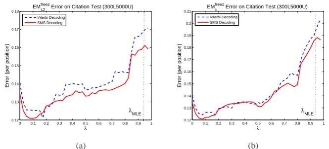
Figure 2: EMλerror rates while increasing the allocation from 0 to 1 by the step size0.025.
to segment the document into fields, and to label each field. In our experiments we use the bibli-ographic citation dataset described in (Peng and McCallum, 2004) (see Fig. 1 for an example of the input and expected label output for this task). This dataset has 500 annotated citations with 13 fields; 5000 unannotated citations were added to it later by (Grenager et al., 2005). The annotated data is split into a 300-document training set, a document development (dev) set, and a 100-document test set7.
We use a first order HMM with the size of hid-den states equal to the number of fields (equal to 13). We freeze the transition probabilities to what has been observed in the labeled data and only learn the emission probabilities. The transition probabilities are kept frozen due to the nature of this task in which the transition information can be learned with very little labeled data, e.g. first start with ’author’ then move to ’title’ and so on. However, the challenging aspect of this dataset is to find the segment spans for each field, which de-pends on learning the emission probabilities, based on the fixed transition probabilities.
At test time, we use both Viterbi (most probable sequence of states) decoding and sequence of most probable states decoding methods, and abbreviate them by Viterbi and SMS respectively. We report results in terms of precision, recall and F-measure for finding the citation fields, as well as accuracy calculated per position, i.e. the ratio of the words labeled correctly for sequences to all of the words. The segment-based precision and recall scores are,
7
From http://www.stanford.edu/grenager/data/unsupie.tgz
of course, lower than the accuracy computed on the per-token basis. However, both these numbers need to be taken into account in order to under-stand performance in the field segmentation task. Each input word sequence in this task is very long (with an average length of 36.7) but the number of fields to be recovered is a small number compar-atively (on average there are 5.4 field segments in a sentence where the average length of a segment is 6.8). Even a few one-word mistakes in finding the full segment span leads to a drastic fall in pre-cision and recall. The situation is quite different from part-of-speech tagging, or even noun-phrase chunking using sequence learning methods. Thus, for this task both the per-token accuracy as well as the segment precision and recall are equally impor-tant in gauging performance.
Smoothing to remove zero components in the starting point is crucial otherwise these features do not generalize well and yet we know that they have been observed in the unlabeled data. We use a sim-ple add-ǫ smoothing, where ǫ is .2 for transition table entries and .05 for the emission table entries. In all experiments, we deal with unknown words in test data by replacing words seen less than 5 times in training by the unknown word token.
5.1 Problems with MLE
MLE chooses to set λ = |L||U+||U| which almost ignores labeled data information and puts all the weight on the unlabeled data8. To see this empir-ically, we show the per position error rates at
dif-8
ferent source allocation for HMMs trained on 300 labeled and 5000 unlabeled sequences for the Ci-tation dataset in Fig. 2(a). For each allocation we have runEMλ algorithm, initialized to smoothed counts from labeled data, until convergence. As the plots show, initially the error decreases asλ in-creases; however, it starts to increase afterλpasses a certain value. MLE has higher error rates com-pared to complete data estimate, and its perfor-mance is far from the best way of combining la-beled and unlala-beled data.
In Fig. 2(b), we have done similar experiment with the difference that for each value of λ, the starting point of the EMλ is the final solution found in the previous value of λ. As seen in the plot, the intermediate local optima have better per-formance compared to the previous experiment, but still the imbalance between labeled and unla-beled data negatively affects the quality of the so-lutions compared to the purely supervised solution. The likelihood surface is non-convex and has many local maxima. Here EM performs hill climb-ing on the likelihood surface, and arguably the re-sulting (locally optimal) model may not reflect the quality of the globally optimal MLE. But we con-jecture that even the MLE model(s) which globally maximize the likelihood may suffer from the prob-lem of the size imbalance between labeled and un-labeled data, since what matters is the influence of unlabeled data on the likelihood. (Chang et. al., 2007) also report on using hard-EM on these datasets9in which the performance degrades com-pared to the purely supervised model.
5.2 Choosingλin Homotopy-based HMM
We analyze different criteria in picking the best value ofλbased on inspection of the continuation path. The following criteria are considered: • monotone: The first iteration in which the monotonicity of the path is changed, or equiva-lently the first iteration in which the determinant ofλ∇Θ˜EM1(Θ)−Iin Algorithm 1 becomes zero (Corduneanu and Jaakkola, 2002).
•minEig: Instead of looking into the determinant
of the above matrix, consider its minimum eigen-value. Across all iterations, choose the one for which this minimum eigenvalue is the lowest. •maxEnt: Choose the iteration whose model puts
the maximum entropy on the labeling distribution for unlabeled data (Ji et al., 2007).
9
In Hard-EM, the probability mass is fully assigned to the most probable label, instead of all possible labels.
The second criterion is new, and experimentally has shown a good performance; it indicates the amount of singularity of a matrix.
100 150 200 250 300 350 400 450 500
0 0.1 0.2 0.3 0.4 0.5 0.6 0.7 0.8 0.9
# Unlabeled Sequences
λ
Best Selected Allocations
monton maxEnt
minEig EM
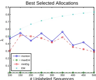
Figure 3: λ values picked by different methods. The size of the labeled data is fixed to 100, and results are averaged over 4 runs. The λ values picked by MaxEnt method for 500 unlabeled ex-amples was .008.
We fix 100 labeled sequences and vary the num-ber of unlabeled sequences from 100 to 500 by a step of 50. All of the experiments are repeated four times with different randomly chosen unla-beled datasets, and the results are the average over four runs. The chosen allocations based on the de-scribed criteria are plotted in Figure 3, and their associated performance measures can be seen in Figure 4.
Figure 3 shows that as the unlabeled data set grows, the reliance of ’minEig’ and ’monotone’ methods on unlabeled data decreases whereas in EM it increases. The ’minEig’ method is more conservative than ’monotone’ in that it usually
chooses smaller λ values. The plots in
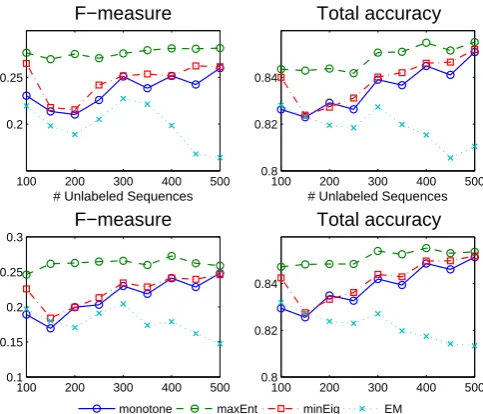
Fig-ure 4 show that homotopy-based HMM always outperforms EM-based HMM. Moreover, ’max-Ent’ method outperforms other ways of picking λ. However, as the size of the unlabeled data in-creases, the three methods tend to have similar per-formances.
5.3 Homotopy v.s. other methods
In the second set of experiments, we compare the performance of the homotopy based method against the competitive methods for picking the value ofλ.
100 200 300 400 500 0.2
0.25
F−measure
# Unlabeled Sequences
100 200 300 400 500 0.8
0.82 0.84
Total accuracy
# Unlabeled Sequences
100 200 300 400 500 0.1
0.15 0.2 0.25 0.3
F−measure
100 200 300 400 500 0.8
0.82 0.84
Total accuracy
monotone maxEnt minEig EM
Figure 4: The comparison of different techniques for choosing the best allocation based on datasets with 100 labeled sequences and varying number of unlabeled sequences. Each figure shows the av-erage over 4 runs. F-measure is calculated based on the segments, and total accuracy is calculated based on tokens in individual positions. The two plots in the top represent Viterbi decoding, and the two plots in the bottom represent SMS decoding.
ofλbased on brute-force search using a fixed step size; afterwards, this value is used to train HMM (based on 200 remaining labeled sequences and unlabeled data). The second competitive method, which we call ’Oracle’, is similar to the previous method except we use the test set as the held out set and all of the 300 labeled sequences as the train-ing set. In a sense, the resulttrain-ing model is the best we can expect from cross validation based on the knowledge of true labels for the test set. Despite the name ’Oracle’, in this setting theλvalue is se-lected based on the log-likelihood criterion, so it is possible that the ’Oracle’ method is outperformed by another method in terms of precision/recall/f-score. Finally, EM is considered as the third base-line.
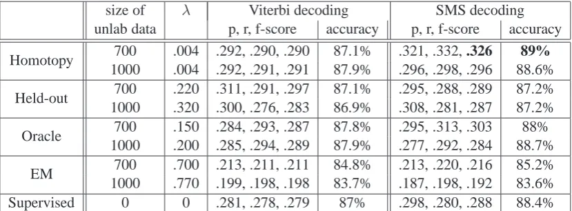
The results are summarized in Table 1. When decoding based on SMS, the homotopy-based HMM outperforms the ’Held-out’ method for all of performance measures, and generally behaves better than the ’Oracle’ method. When decoding based on Viterbi, the accuracy of the homotopy-based HMM is better than ’Held-out’ and is in the same range as the ’Oracle’; the three meth-ods have roughly the same f-score. The λ value
found by Homotopy gives a small weight to unla-beled data, and so it might seem that it is ignoring the unlabeled data. This is not the case, even with a small weight the unlabeled data has an impact, as can be seen in the comparison with the purely Supervised baseline in Table 1 where the Homo-topy method outperforms the Supervised baseline by more than 3.5 points of f-score with
SMS-decoding. Homotopy-based HMM with
SMS-decoding outperforms all of the other methods. We noticed that accuracy was better for 700 un-labeled examples in this dataset, and so we include those results as well in Table 1. We observed some noise in unlabeled sequences; so as the size of the unlabeled data set grows, this noise increases as well. In addition to finding the right balance be-tween labeled and unlabeled data, this is another factor in semi-supervised learning. For each par-ticular unlabeled dataset size (we experimented us-ing 300 to 1000 unlabeled data with a step size of 100) the Homotopy method outperforms the other alternatives.
6 Related Previous Work
Homotopy based parameter estimation was orig-inally proposed in (Corduneanu and Jaakkola, 2002) for Na¨ıve Bayes models and mixture of Gaussians, and (Ji et al., 2007) used it for HMM-based sequence classification which means that an input sequence x is classified into a class label y ∈ {1, . . . , k} (the class label is not structured, i.e. not a sequence of tags). The classification is done using a collection ofkHMMs by computing
Pr(x, y | Θy) which sums over all states in each
HMMΘy for inputx. The algorithms in (Ji et al., 2007) could be adapted to the task of sequence la-beling, but we argue that our algorithms provide a straightforward and direct solution.
di-size of λ Viterbi decoding SMS decoding
unlab data p, r, f-score accuracy p, r, f-score accuracy
Homotopy 700 .004 .292, .290, .290 87.1% .321, .332, .326 89%
1000 .004 .292, .291, .291 87.9% .296, .298, .296 88.6%
Held-out 700 .220 .311, .291, .297 87.1% .295, .288, .289 87.2%
1000 .320 .300, .276, .283 86.9% .308, .281, .287 87.2%
Oracle 700 .150 .284, .293, .287 87.8% .295, .313, .303 88%
1000 .200 .285, .294, .289 87.9% .277, .292, .284 88.7%
EM 700 .700 .213, .211, .211 84.8% .213, .220, .216 85.2%
1000 .770 .199, .198, .198 83.7% .187, .198, .192 83.6%
Supervised 0 0 .281, .278, .279 87% .298, .280, .288 88.4%
Table 1: Results using entire labeled data with segment precision/recall/f-score and token based accuracy.
rect numerical comparison impossible. (Peng and McCallum, 2004) used only labeled data to train conditional random fields and HMMs with second order state transitions where they allow observa-tion in each posiobserva-tion to depend on the current state as well as observation of the previous position.
7 Conclusion
In many NLP tasks, the addition of unlabeled data to labeled data can decrease the performance on that task. This is often because the unlabeled data can overwhelm the information obtained from the labeled data. In this paper, we have described a methodology and provided efficient algorithms for an approach that attempts to ensure that unlabeled data does not hurt performance. The experimen-tal results show that homotopy-based training per-forms better than other commonly used compet-itive methods. We plan to explore faster ways for computing the (approximate) covariance ma-trix, e.g., label sequences can be sampled from P(y|x,Θ) and an approximation of the covari-ance matrix can be computed based on these sam-ples. Also, it is possible to compute the covariance matrix in polynomial-time for labels which have richer interdependencies such as those generated by a context free grammars (Haffari and Sarkar, 2008). Finally, in Algorithm 1 we used a fixed step size; the number of iterations in the homo-topy path following can be reduced greatly with adaptive step size methods (Allgower and Georg, 1993).
References
E. L. Allgower, K. Georg 1993. Continuation and Path Following, Acta Numerica, 2:1-64.
M. Chang and L. Ratinov and D. Roth. 2007. Guiding
Semi-Supervision with Constraint-Driven Learning, ACL 2007.
M. Collins 2005. Notes on the EM Algorithm, NLP course notes, MIT.
A. Corduneanu. 2002. Stable Mixing of Complete and Incomplete Information, Masters Thesis, MIT.
A. Corduneanu and T. Jaakkola. 2002. Continuation Methods for Mixing Heterogeneous Sources, UAI 2002.
T. Grenager, D. Klein, and C. Manning. 2005. Unsu-pervised Learning of Field Segmentation Models for Information Extraction, ACL 2005.
G. Haffari and A. Sarkar. 2008. A Continuation Method for Semi-supervised Learning in Product of Multinomials Models, Technical Report. Simon Fraser University. School of Computing Science.
K. Lari, and S. Young. 1990. The estimation of stochastic context-free grammars using the inside-outside algorithm, Computer Speech and Language (4).
S. Ji, L. Watson and L. Carin. 2007. Semi-Supervised Learning of Hidden Markov Models via a Homotopy Method, manuscript.
B. Merialdo. 1993. Tagging English text with a proba-bilistic model, Computational Linguistics
K. Nigam, A. McCallum, S. Thrun and T. Mitchell. 2000. Text Classification from Labeled and Unla-beled Documents using EM, Machine Learning, 39. p. 103-134.
F. Peng and A. McCallum. 2004. Accurate Information Extraction from Research Papers using Conditional Random Fields, HLT-NAACL 2004.
L. Rabiner. 1989. A Tutorial on Hidden Markov Mod-els and Selected Applications in Speech Recogni-tion, Proc. of the IEEE, 77(2).