Link performance of the time offset transmitted reference system

University of Twenty

Faculty of Electrical Engineering

Chair for Telecommunication Engineering

Link performance of the time offset

transmitted reference system

By

A. Bekkaoui

Thesis of a Master’s Assignment

Executed from November 2003 till June 2004 Supervisor: Prof. Dr. Ir. J.C. Haartsen Advisors: Prof. Dr. Ir. W. Van Etten

Summary

There has been an interest in recent years in exploiting noise modulation for the transmission of analog and digital information in radio communications. Because of their broad bandwidth noise signals can be used to spread the information signal letting us to transmit an ultra wideband (UWB) signal. Noise communication can use a delay line both at the transmitter and at the receiver. To distinguish between the modulated signal and the reference signal the time offset is much larger then the coherence time of the noise carrier.

In this thesis the performance of the time offset transmitted reference is determined in the presence of the AWGN in terms of signal-to-beat noise ratio (SNR) and bit error rate (BER). The broadband noise carrier is modeled as a Gaussian distribution. The result is a simple expression where the beat-noise and the number of users are involved.

By the study of a band limited broadband noise carrier, the bit error rate is determined as a function of

0 b E

N . It is proved that the number of users and the processing gain G limits the BER. Moreover, the BER degrades as the number of users increases. Also it is shown that the BER develops an error floor and this increases rapidly with the number of users. Theoretically we found that the BER at fixed

0 b E

N attains its minimum at a certain processing gain G.

It was shown that narrowband interferences could jam completely the information signal. Significant improvement in performance can be obtained if Manchester line coding is used. In a multipath environment, the difference between each pair of multipath delays should be larger than the coherence time of the noise carrier.

Table of contents

List of symbols ... 8

List of abbreviations... 9

List of operators and special functions ... 10

1

Introduction ... 11

1.1 Ultra wideband technology ...11

1.2 Noise signals ...14

1.3 Conventional Transmitted reference (TR) systems...15

1.4 New system using transmitted reference principle ...16

1.5 Research goal ...18

1.6 Thesis organization ...18

2

Time offset transmitted reference principle... 19

2.1 Spread spectrum communication ...19

2.2 Time offset transmitted reference architecture...20

2.2.1 Transmitter ...20

2.2.2 Receiver...22

3

Link performance in AWGN for one user... 25

3.1 Transmitter ...25

3.2 Receiver input ...26

3.3 Mixer output...27

3.3.1 Instantaneous mixer output ...28

3.3.2 Average mixer output...30

3.4 The time offset transmitted reference signal-to-beat noise ratio...32

3.4.1 Mixer beat noise power spectral density ...33

3.4.2 Integrate and dump filter output...33

3.4.3 Signal-to-beat noise ratio ...35

3.5 Detection probability...36

3.6 Evaluation for band limited spectrally flat noise carrier ...36

3.6.2 Numerical evaluation ...40

4

Link performance for multiple users ... 45

4.1 Mixer output...45

4.1.1 Instantaneous mixer output ...45

4.1.2 The average of the mixer output ...48

4.2 Power spectral density of the beat noise in the information band...50

4.3 Signal-to-beat noise ratio at the integrate and dump filter output...51

4.4 Evaluation for band limited spectrally flat noise carriers ...52

4.4.1 Numerical evaluation ...54

5

Multipath effect and narrowband interference ... 59

5.1 Multipath effect ...59

5.1.1 The mean value ...60

5.2 Narrowband interference...63

5.2.1 Narrow band suppression using Manchester line code ...66

6

Simulation results ... 69

6.1 Simulation model ...69

6.1.1 The Gaussian noise generator ...69

6.1.2 Data signal generator...70

6.1.3 Modulator ...70

6.1.4 The additive white Gaussian noise block...70

6.1.5 Integer delay...71

6.1.6 Integrate and dump filter ...71

6.1.7 Decoder ...72

6.1.8 Error rate calculation block set...72

6.2 Simulation setup and configurations ...72

6.2.1 System with one transmitter and one receiver ...73

6.2.2 System with two transmitters and two receivers...74

6.2.3 System with four users ...74

6.2.4 Error floor...76

7

Conclusions and recommendations ... 77

7.1 Conclusions ...77

Appendix A

Calculation on the time offset transmitted reference

system with one transmitter and one receiver ... 79

Appendix A1 Calculation of the average mixer output ...79

Appendix A2 Calculation of the mixer output autocorrelation function ...80

Appendix A3 Calculation of the mixer output power spectral density ...87

Appendix B

Calculation on the time offset transmitted reference with

multiple transmitters and receivers... 91

Appendix B1 Calculation of the mixer output autocorrelation function...91

List of symbols

( )

A t The amplitude of the narrowband signal B Bandwidth of the noise carrier

c(t) Pseudo noise signal b

E Received bit energy

f: Frequency variable used as an argument of power spectral density functions 0

f The carrier frequency for the narrowband signal G processing gain

( )

J t Narrowband interference signal

H(f): transfer function of the broadband noise filter. h(t) The impulse function of the broadband filter

2

h (t) The time-reversed version of ( )h t i

m: Data bit sent by user i ˆ_i

m: Detected data bit M Number of transmitters

n(t): Additive white Gaussian noise N Number of multipath

0

N Power spectral density of the AWGN. e

P Bit error rate ( )

nn

R τ Autocorrelation function of n(t) ( )

xx

R τ Autocorrelation function of x(t) s(t): transmitted signal

SNR signal-to-beat noise ratio ( )

nn

S f Power spectral density function of the random process n(t) ( )

xx

S f Power spectral density function of the random process x(t) t: Time variable used as an argument of time signal

Tb: Bite time

i

J

v The integrator output resulting only from the narrowband filter J t

( )

w(t) Broadband filter output

( )

J

w t The broadband filter output resulting from the narrowband signal J t

( )

x(t): Noise carrier y(t): Received signal z(t) Mixer output

( ) J

z t The mixer output component resulting from the narrowband signal J t

( )

i

α Time variable used in integrals

( )

i t

γ Attenuation factor for the i-th path

τ : Time difference variable used as an argument of correlation functions c

τ Coherence time

i

τ : Time offset for user i r

τ The time offset at the receiver.

ν Frequency variable used in integrators

i

κ Propagation delay for the i-th path ( )t

φ The phase of the narrowband signal

List of abbreviations

AWGN Additive white Gaussian noise BER Bit error rate

CDSK Correlation delay shift keying DCSK Differential chaos shift keying FCC Federal communication commission NRZ Non return to zero

List of operators and special functions

⊗: Convolution operator

{ }x

Ε Mean value of the random variable x

x Absolute value of variable x ( )t

1 Introduction

The basics of radio transceivers have hardly changed since the first radio communication experiments carried out by Marconi around 1900. In general radio transceivers consist of tuned circuits with limited bandwidth. Sinusoidal waveforms are used as carriers to transport the user information. Hence the transmitter implementation contains expensive filters and oscillators. Moreover the radio spectrum is limited and there are a lot of users. Therefore multiple access techniques are used to allow many mobile users to share the finite amount of the radio spectrum simultaneously. Examples of radio multiple access techniques are Time Division Multiple Access (TDMA), Frequency Division Multiple Access (FDMA), and Code Division Multiple Access CDMA. These techniques are based on absolute frequency, time, or code sequence, which must be known both at the receiver and the transmitter. All these are extensively discussed in [1]. The conventional radio transmission has some disadvantages. It requires a lot of co-ordination between the transmitter and the receiver. Moreover the narrow bandwidth limits the applications used in the mobile telecommunications. This situation pushed a lot of research groups to look for new communications techniques to increase for instance the radio channel bandwidth and therefore the bit rate of the information signal, or to make the radio transceiver cheaper, or to implement a transceiver to fulfill the two previous requirements.

Recently a new modulation technique has been investigated which breaks with the conventional tuned transceiver and which is not based on a sine waveform carrier. This technique is called Ultra Wideband transmission (UWB). The next section will give a brief description of the advantages of UWB transmission.

1.1 Ultra wideband technology

UWB is defined by the Federal Communication Commission (FCC) as: the bandwidth of the UWB signal is at least 20% of the center frequency or more than 500 MHz [2].

indoor applications with high-speed data transmissions. It is expected that the UWB technology can deliver wireless connections as fast as 100Mbps.

UWB does have many advantages such as:

• By using UWB technique high data rate can be reached.

• Simple RF architecture [3].

• UWB doesn’t use sine waves as carriers. Therefore the transceiver doest not contain expensive filters and oscillators. Not using sine waves can also results in no multipath cancellation effects. Non-sinusoidal nature of waves prevents cancellation of waves that occurs when waves are reflected and meet partially or totally out of phase with one another.

• The UWB radio transceiver can result in a cheap implementation. Transceivers will be low cost because the electronics can be completely integrated onto a CMOS.

• Low power spectral density: the low power spectral density enables the UWB system to co-exist with other communication systems [3] (Figure 1.1).

Figure 1.1:UWB power spectral density showing the co-existence of the UWB systems with other communication systems.

Figure 1.2: Allowed UWB emission for indoor and outdoor telecommunication

1

3

1

4

-All o w ed e mi ss io n [d B

1 GHz 10 GHz

-75 -70 -65 -60 -55 -50 -45

-40 _Outdoor

Indoor

dBm/MHz

Telecommunication

The modulation technique proposed for UWB by most research groups is based on ultra-short pulses. It uses pulse position modulation of very short duration pulses. The pulse width is between 0.1 nanosecond and 1.5 nanosecond. To enable multiple access in radio impulse modulation time hopping is used. However, a modulation alternative is to use broadband noise signals. This thesis is about using noise signals for spread spectrum communication. To put this work into context, we will first briefly discuss noise signals.

1.2 Noise signals

Noise signals are bounded, and have aperiodic behavior that exhibits sensitivity to initial conditions. This sensitivity can be demonstrated by giving two very close initial states to a chaotic map; After a few iterations, the two resulting sequences will look completely decorrelated [6]. That means that the time evolution of a noise system, while governed by strictly deterministic equations, is impossible to predict beyond extremely small time scales. Noise is extremely common in nature. In fact, many common non-linear dynamical systems are often found to exhibit chaotic behavior for a certain parameter ranges. In electrical and electronic systems, there are many circuit components that are inherently non-linear, such as diodes, transistors, switches and oscillators. Circuits containing these elements often display chaotic behavior. The inherently broadband nature of noise signals has made them promising for spread spectrum communication systems. Moreover an advantage of a noise-based communication system is a less complicated circuitry in comparison with conventional spread spectrum approaches. Consequently, the weight and volume requirements of the devices are reduced and efficiency is increased. It may be possible to put a complete transmitter or receiver on one small chip [6].

1.3 Conventional Transmitted reference (TR) systems.

This section will give a brief description of the conventional transmitted reference schemes and some disadvantages using these schemes.

The conventional transmitted reference system was studied for the first time in the beginning of the 1950s. Simultaneously at M.I.T and at the USA army some experimental works were done. The conventional transmitted reference systems accomplish spread spectrum operation by transmitting two versions of a wideband signal, unpredictable carrier, one modulated by data and the other unmodulated (Figure 1.3) [9]. These two signals are transmitted separately over two different channels (one may be displaced in frequency from the other). The two signals, being separately recovered by the receiver, are the input for a correlator detector, which recovers the data [9]. The wideband carrier in a conventional transmitted reference system may be random, wideband noise source, unknown by the transmitter and the receiver until the instant it is generated for use in communication.

The conventional transmitted reference does have fundamental weaknesses:

• The available bandwidth is divided between the two signals, the reference and the modulated signal. This system is not bandwidth efficient because half of the bandwidth is not used to transport data.

• The transmitted reference system’s two channels may be difficult to match [9].

• Any listener who has access to both transmitted signals easily determines the data.

• The conventional transmitted reference uses two transmitters and two receivers and that makes the cost for the radio implementation expensive.

Figure 1.3: Conventional Transmitted Reference system [9]

1.4 New system using transmitted reference principle

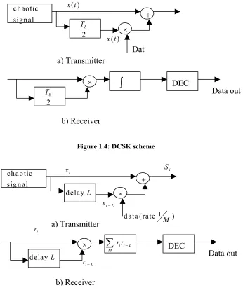
The spread-spectrum strategy used in the conventional transmitted reference employing two channels can be more efficiently used if the two signals are sent over one channel. One of the most popular solutions proposed is the differential chaos shift keying DCSK [10]. The structure of a typical DCSK transmitter and receiver is shown in Figure 1.4 [10]. A reference chaotic waveform ( )x t is transmitted during the first half of each data bit. If the bit is a ‘1’, ( )x t is transmitted again during the second half. If the bit is a ‘0’, −x t( ) is transmitted. At the receiver, the signal is delayed by half a bit period and correlated with the undelayed signal to get the decision variable for producing the output data stream. In DCSK, part of the information associated with the chaotic carrier remains unexploited. In fact, the total channel capacity is shared between the reference signal that is transmitted during the first half of the bit period and the modulated signal that is transmitted during the second half of the bit period. A multiple-access technique for the use with DCSK is proposed and analyzed in [12].

To be able to use the whole channel capacity another modulation technique is proposed. This technique is called correlation delay shift keying CDSK Figure 1.5 [10]. In CDSK, instead of the sequence transmission of the modulated chaotic signal and the reference, as it is done in DCSK, the two are added together with a certain time delay. This permits a continuous operation of the transmitter and makes the transmitted signal more homogenous.

data

noise

Mod Demo data

( ) d t

( )

x t _{x tˆ( )}

ˆ( ) d t

Tx

Tx Rx

Figure 1.4: DCSK scheme

Figure 1.5: CDSK scheme [10]

This thesis will investigate a similar scheme as CDSK. This technique could be called time offset transmitted reference. The transmitted reference and the modulated signal are combined at the transmitter and transmitted over one channel. The differences between the two schemes can be summarized in two points: the noise signal in our work has a Gaussian distribution and the chaotic signal scheme discussed in [10] used a symmetric tent map signals and has a uniform distribution. The time delay used in the CDSK scheme is longer than the bit time to be sure that the cross-correlation between the modulated signal and the reference is minimum. But in our work the time delay is much smaller than the bit time.

×

2

b

T

∫

DEC Data out

a) Transmitter

b) Receiver

+ ×

2

b

T

Dat

chaotic signal

( )

x t

( )

x t

× i i L _DEC

M

r r₋

∑

Data out a) Transmitter

b) Receiver

+ ×

delay L

ch ao tic sign al

i

x

i L

x₋

1 d ata ( rate _M )

i

S

d elay L

i

r

i L

At the telecommunication Engineering group at the University of Twente another UWB transmission technique is studied. The system is called frequency offset division multiple access FODMA [11]. This technique is based on a frequency offset rather than the time offset and uses also noise signals as a carrier.

1.5 Research goal

The goal of this research is to study the architecture and the principle of the time offset transmitted reference system and to determine the link performance of the time offset transmitted reference scheme taking into account the auto-correlation terms in the case of one user. The link performance for multiple users will also be determined, where the cross-correlation and the number of users are taken into account. The work contains an analytical part and a simulation part and a comparison between the achieved results.

1.6 Thesis organization

2 Time offset transmitted reference principle

This thesis is about using noise signals for spread spectrum communication. To put this work into context, we will first briefly discuss spread spectrum communication. Then we will discuss a detailed description of the time offset transmitted reference scheme and the principle of this technique.

2.1 Spread spectrum communication

Spread spectrum communication aims at using a transmitted signal designed to have a bandwidth much larger than the minimum required to transmit data at a given rate. The process of increasing the bandwidth of the data signal before transmitting it is called spreading. Conventional spreading techniques fall into two basic classes:

1. Direct Sequence Spread Spectrum (DS-SS): a high-speed pseudo-random binary sequence known as the spreading code is multiplied with the data signal to increase its bandwidth.

2. Frequency Hopping Spread Spectrum (FH-SS): the data signal is modulated by a carrier whose frequency is varied over time by a frequency synthesizer under the control of a high-speed pseudo-random binary sequence.

At the receiver, the signal is subjected to despreading in order to reduce the bandwidth to the original value. This is typically performed by a correlation. Based on the correlation method, the main types of spread spectrum systems are:

1. Stored Reference (SR) systems: in such systems, the transmitter and the receiver are synchronized, the spreading pseudo-random binary sequence by the transmitter is regenerated at the receiver and the received signal is correlated with it to recover the transmitted data. CDMA is stored reference system.

In general, transmitted reference communication is advantageous when transmitting through an unknown channel that severely distorts the transmitted waveforms making the use of a stored, phase synchronous filter problematic. The reference, because it passes through the same channel as the modulated signal, is distorted in the same way as the carrier of the modulated signal. That means that no synchronization is needed between the reference signal and the modulated signal. The next section will investigate the time offset transmitted reference system using a broadband noise signal and based on transmitted reference.

2.2 Time offset transmitted reference architecture

2.2.1 Transmitter

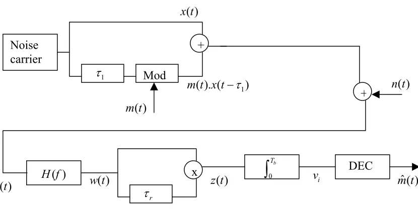
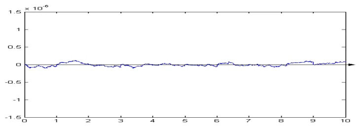
Figure 2.1 shows the architecture of the time offset transmitted reference scheme. The transmitter generates a broadband noise signal with a mean value equal to zero (Figure 2.2). To make difference between the AWGN and the generated signal at the receiver, we will call the generated signal noise carrier. The signal is split into two branches. The signal in the upper branch is used as a reference for the modulated signal. The signal in the second branch is delayed by a time offset equal toτ₁ (we will see in the next chapter that the time offset τ₁ should be greater then the coherence time of the noise carrier). The delayed signal is modulated by the information signal. The modulation involves a multiplication of the noise carrier by the information-signal. The modulator is assumed to be an ideal multiplier. That means that the output signal is the product of the incoming noise carrier and the information signal. The information-signal is assumed to be a rectangular polar NRZ signal m(t) (Figure 2.3), which takes the values +1 and –1. The two signals coming from the two branches are combined and then transmitted. To be able to detect the information signal at the receiver the time offset τ₁ should be much larger than the coherence time of the noise carrier. In this case the cross correlation between the noise carrier and its shifted version is almost equal to zero [16].

Figure 2.1: The time offset transmitted reference scheme

Figure 2.2: Noise carrier with a mean value equal to zero

Figure 2.3: Information signal

t +

1

τ

Noise carrier

( ) x t

1 ( ). ( ) m t x t−τ

( ) m t

Mod

+ n t( )

x r

τ

0 b T

∫

( ) y t

DEC ( )

w t z t( ) vi m tˆ ( )

2.2.2 Receiver

The transmitted signal will be corrupted by additive white Gaussian noise (White noise cannot exist in real life. However, white noise approximates random processes encountered in nature). At the receiver, the received signal passes through a wideband filter to limit the effect of the additive white Gaussian noise. The bandwidth of the broadband filter should be at least equal to the bandwidth of the noise carrier. The signal coming from the broadband filter is split into two signals; the signal in the lower branch is delayed by a time offset equal to τ_r and then multiplied by the original version of the received signal. We will see in the next chapter that if the absolute value of the difference between the time offsets at the receiver τ_r and the at the transmitter τ₁ is much smaller than the coherence time of the noise carrier then the information signal is de-spread directly to base band at the mixer output (Figure 2.4). After low-pass filtering the information signal remains. Figure 2.5 shows the integrator output. Otherwise, if the absolute value of the difference between the time offsets at the receiver τ_r and the at the transmitter τ₁ is much larger than the coherence time of the noise then the signal at the mixer output is a noise with a mean value equal to zero (Figure 2.6). Figure 2.7 shows the integrator output. It is quite impossible for the receiver to take the right decision about the transmitted bit. The entire de-spreading operation includes only a delay line and a correlator to demodulate the signal.

Figure 2.5: Integrator output if the delays at both the receiver and the transmitter are equal

Figure 2.6: The mixer output if the delays at both the receiver and the transmitter are different

3 Link performance in AWGN for one user

In chapter 2 we described the architecture of the time offset transmitted reference system and its principles. This chapter will investigate the link performance of the time offset transmitted reference system, when it is corrupted by AWGN. In this chapter we will study the case of one transmitter and one receiver. The last section will investigate an example in detail.

3.1 Transmitter

In this section we will determine the signal output of the transmitter.

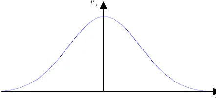
Figure 3.1 illustrates the transmitter architecture. The transmitter generates a noise carrier. This noise carrier is unknown by the transmitter and the receiver until the instant it is generated for use in communication. We assume that the noise carrier has a Gaussian distribution and its mean value is equal to zero (Figure 3.2).

Figure 3.1: The time offset transmitted reference transmitter

Figure 3.2: PDF of the Gaussian distribution with a mean value equal to zero

x

P

x ( )

i

m t 1

τ

+ ( )

x t

1

( ). ( )

i

m t x t−τ

( )

s t

noise carrier

The signal in the lower branch in the interval 0≤ ≤t T_b can be written as: 1

( ). ( ) 0

i b

m t x t−τ ≤ ≤t T (3-1)

( ) i

m t Data signal sent by the user ( )

x t Noise carrier 1

τ Time offset used by the transmitter

In our calculation we will assume that the bit time Tb is large enough to assume that all signals in

the system are quasi stationary during one bit time. Thus the bit signal m t_i( ) is assumed to be constant. Equation (3-1) can be written as

1

. ( ) 0

i b

m x t−τ ≤ ≤t T (3-2)

We assume also that the time offset τ₁ is much smaller than the bit time Tb.

Combining the two signals coming from the two branches, the output of the transmitter can be written as:

1

( ) ( ) _i. ( ) 0 _b

s t =x t +m x t−τ ≤ ≤t T (3-3)

3.2 Receiver input

The channel is assumed to corrupt the signal by the addition of white Gaussian noise (AWGN) as illustrated in Figure 3.3. We assume that the channel causes no attenuation, no delay, and no distortion. The received signal may be expressed as:

( ) ( ) ( )

y t =s t +n t (3-4)

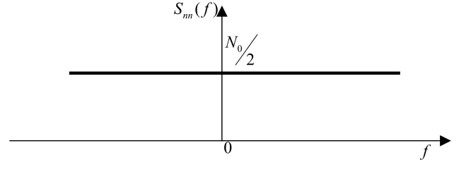
Where n(t) denotes the Additive White Gaussian Noise (AWGN) process having a mean value equal to zero and having a double sided spectral density

2

0

N

W / Hz (Figure 3.4). ( )s t denotes the transmitted signal.

Substituting equation (3-3) in equation (3-4) we get: )

( ) ( . ) ( )

(t x t m x t n t

Figure 3.3: Received signal passed through AWGN channel

Figure 3.4: Power spectral density of the AWGN

3.3 Mixer output

It is convenient to divide the receiver into two parts, the signal demodulator and the signal detector, as shown in Figure 3.5. The function of the demodulator is to convert the received waveform to a base band signal. The function of the detector is to decide which bit was transmitted based on the value v_i.

Figure 3.5: The receiver configuration

+ ( ) n t

( ) s t

( )

y t

Received signal Transmitted signal

AWGN

Received signal

( )

y t

i

v

m

ˆ

_i

Output decision

Demodulator _Detector

( ) nn S f

0 2 N

f

Figure 3.6: The time offset transmitted reference demodulator

Figure 3.6 shows the architecture of the demodulator. It contains a broadband filter, a delay line, a mixer, and an integrate and dump filter. The integration time is equal to the information bit time Tb. Based on the observation of v_i, we will determine the link performance of the time offset

transmitted reference system. To reach this goal different steps should be followed. First, we will determine the mixer instantaneous output z(t) and its mean value. Then we will determine the covariance of the mixer output z(t). Second, we will determine the power spectral density of the mixer output by Fourier transforming the covariance. The third step is to determine the noise in the information band. The latter step in the calculation of the link performance is to find out the distribution of the integrate and dump filter output v_i.

3.3.1 Instantaneous mixer output

In this section we will determine the instantaneous mixer output z(t). The input signal y(t) to the receiver is given by (3-5). The signal passes through the broadband filter to remove all high frequencies. The output of the broadband filter is given by:

) ( ) ( )

(t y t h t

w = ⊗ (3-6)

⊗: Convolution operator

h(t) the impulse function of the broadband filter We write out the convolution

( ) ( ). ( )d

w t ∞ y t α h α α

−∞

=

∫

− (3-7)

The signal coming from the filter will be delayed by a time offset equal to τ_r and then mixed with the original received signal. The mixer output z(t) can be written as:

( ) ( ). ( _r)

z t =w t w t−τ (3-8)

0 T

∫

x r

τ

( )

H f w t( )

( ) z t

i v ( )

z(t) is the instantaneous mixer output. r

τ is the time offset at the receiver.

We substitute w(t)and (w t−τ_r) by their expression given by (3-7), so equation (3-8) becomes:

1 1 1 2 2 2

( ) ( ). ( )d ( _r ). ( )d

z t ∞ y t α hα α ∞ y t τ α hα α

−∞ −∞

=

∫

−

∫

− − (3-9)

The product of the two integrals in equation (3-9) can be written as a double integral, which gives:

1 2 1 2 2 1

( ) ( ). ( _r ). ( ). ( )d d

z t ∞ ∞ y t α y t τ α hα hα α α

−∞ −∞

=

∫ ∫

− − − (3-10)

If we substitute y(t−α₁)and y t( − −τ_r α₂) by their expressions given by equation (3-5), equation (3-10) can be written as:

{

}

{

}

1 2 1 1 1 1

2 2 1 2 1 2

( ) ( ). ( ). ( ) . ( ) ( )

. ( ) . ( ) ( ) d d

i

r i r r

z t h h x t m x t n t

x t m x t n t

α α α α τ α

α τ α τ τ α τ α α

∞ ∞

−∞ −∞

= − + − − + −

− − + − − − + − −

∫ ∫

(3-11)

Writing out the product, equation (3-11) can be written as:

1 2

1 2 1

1 2

1 1 2

1 2 1 1 2 1

1 1 2

1 2

1 2 1

( ). ( )

. ( ). ( )

( ). ( )

. ( ). ( )

( ) ( ). ( ) . . ( ). ( )

. ( ). ( )

( ). ( )

. ( ). ( r

i r

r

i r

i i r

i r

r i

x t x t m x t x t x t n t m x t x t

z t h h m m x t x t

m x t n t n t x t m n t x t

α α τ

α α τ τ

α α τ

α τ α τ

α α α τ α τ τ

α τ α τ

α α τ

α α τ

− − −

+ − − − −

+ − − −

+ − − − −

= + − − − − −

+ − − − −

+ − − −

+ − − − −

1 2

1 2

d d

)

( ). ( )

r r n t n t

α α

τ

α α τ

∞ ∞

−∞ −∞

 

 

 

 

 

 

 

 

 

 

 

 

 

_{+ − − −} 

 

∫ ∫

_(3-12)

1 2 1 2 1 2

1 2 1 2 1 1 2

1 2 1 2 1 2

1 2 1 1 2

( ) ( ). ( ) ( ). ( )d d

. ( ). ( ) ( ). ( )d d

( ). ( ) ( ). ( )d d

. ( ). ( ) ( ). ( )

r

i r

r

i r

z t h h x t x t

m h h x t x t

h h x t n t

m h h x t x t

α α α α τ α α α α α α τ τ α α α α α α τ α α α α α τ α τ ∞ ∞ −∞ −∞ ∞ ∞ −∞ −∞ ∞ ∞ −∞ −∞ ∞ −∞ = − − − + − − − − + − − − + − − − −

∫ ∫

∫ ∫

∫ ∫

∫

1 2

1 2 1 1 2 1 1 2

1 2 1 1 2 1 2

1 2 1 2 1 2

1 2

d d

. ( ). ( ) ( ). ( )d d

. ( ). ( ). ( ). ( )d d

( ). ( ) ( ). ( )d d

. ( ). ( )

i i r

i r

r i

m m h h x t x t

m h h x t n t

h h n t x t

m h h n

α α α α α τ α τ τ α α α α α τ α τ α α α α α α τ α α α α ∞ −∞ ∞ ∞ −∞ −∞ ∞ ∞ −∞ −∞ ∞ ∞ −∞ −∞ + − − − − − + − − − − + − − − +

∫

∫ ∫

∫ ∫

∫ ∫

1 2 1 1 2

1 2 1 2 1 2

( ). ( )d d

( ). ( ) ( ). ( )d d

r r

t x t

h h n t n t

α α τ τ α α α α α α τ α α ∞ ∞ −∞ −∞ ∞ ∞ −∞ −∞ − − − − + − − −

∫ ∫

∫ ∫

(3-13)

3.3.2 Average mixer output

The average mixer output z(t) can be found by taking the expected value of z(t) given in equation (3-13).

{ }

1 2 1 2 1 1 2

1 2 1 2 1 1 2

1 2 1 2 1 1 2 1 2 1 1 2 1 1 2

( ). ( ) ( ). ( )d d

. ( ). ( ) ( ). ( 2 )d d

( ). ( ) ( ). ( )d d

. ( ). ( ) ( ). ( )d d

( ) . (

i

i i i

h h x t x t

m h h x t x t

h h x t n t

m h h x t x t

z t m m h

α α α α τ α α α α α α τ α α α α α α τ α α α α α τ α τ α α ∞ ∞ −∞ −∞ ∞ ∞ −∞ −∞ ∞ ∞ −∞ −∞ ∞ ∞ −∞ −∞ − − − + − − − + − − − + − − − − Ε = Ε +

∫ ∫

∫ ∫

∫ ∫

∫ ∫

1 2 1 1 2 1 1 2 1 2 1 1 2 1 1 2 1 2 1 2 1 1 2

1 2 1 2 1 1 2

1 2

). ( ) ( ). ( 2 )d d

. ( ). ( ). ( ). ( )d d

( ). ( ) ( ). ( )d d

. ( ). ( ) ( ). ( 2 )d d

( ). ( )

i

i

h x t x t

m h h x t n t

h h n t x t

m h h n t x t

h h α α α τ α τ α α α α α τ α τ α α α α α α τ α α α α α α τ α α α α ∞ ∞ −∞ −∞ ∞ ∞ −∞ −∞ ∞ ∞ −∞ −∞ ∞ ∞ −∞ −∞ − − − − + − − − − + − − − + − − − +

∫ ∫

∫ ∫

∫ ∫

∫ ∫

1 2 1 1 2

( ). ( )d d

n t α n t α τ α α

∞ ∞ −∞ −∞                                          _{− − −}    

∫ ∫

 (3-14)

Since taking the expected value of an expression is a linear operation, we can interchange the order of integration and taking the expected value. The information bit time Tb is large in

1 2 1 2 1 2

1 2 1 2 1 1 2

1 2 1 2 1 2

1

{ ( )} ( ). ( ) { ( ). ( )}d d

. ( ). ( ) { ( ). ( )}d d

( ). ( ) { ( ). ( )}d d

. ( ). (

r

i r

r i

z t h h x t x t

m h h x t x t

h h x t n t

m h h

α α α α τ α α α α α α τ τ α α α α α α τ α α α α ∞ ∞ −∞ −∞ ∞ ∞ −∞ −∞ ∞ ∞ −∞ −∞ Ε = Ε − − − + Ε − − − − + Ε − − − +

∫ ∫

∫ ∫

∫ ∫

2 1 1 2 1 2

1 2 1 1 2 1 1 2

1 2 1 1 2 1 2

1 2

) { ( ). ( )}d d

. ( ). ( ) { ( ). ( )}d d

. ( ). ( ). { ( ). ( )}d d

( ). ( ) {

r

i i r

i r

x t x t

m m h h x t x t

m h h x t n t

h h n

α τ α τ α α α α α τ α τ τ α α α α α τ α τ α α α α ∞ ∞ −∞ −∞ ∞ ∞ −∞ −∞ ∞ ∞ −∞ −∞ Ε − − − − + Ε − − − − − + Ε − − − − + Ε

∫ ∫

∫ ∫

∫ ∫

1 2 1 2

1 2 1 2 1 1 2

1 2 1 2 1 2

( ). ( )}d d

. ( ). ( ) { ( ). ( )}d d

( ). ( ) { ( ). ( )}d d

r

i r

r

t x t

m h h n t x t

h h n t n t

α α τ α α α α α α τ τ α α α α α α τ α α ∞ ∞ −∞ −∞ ∞ ∞ −∞ −∞ ∞ ∞ −∞ −∞ − − − + Ε − − − − + Ε − − −

∫ ∫

∫ ∫

∫ ∫

(3-15) ) (t

m_i is polar non-return to zero. Therefore m_i.m_i =1 )

(t

x and )n(t are two stationary signals, therefore

1 2 1 2

{ ( ). ( )}x t x t R t_xx( t )

Ε = −

1 2 1 2

{ ( ). ( )}n t n t R t_nn( t )

Ε = −

) (t

x and )n(t are mutually independent, therefore the cross correlation between them is equal to zero. Taking into account the previous properties expression (3-15) can be reduced to:

1 2 1 2 1 2

1 2 1 2 1 1 2 1 2 1 2 1 1 2

1 2 1 2

{ ( )} ( ). ( ) ( )}d d

. ( ). ( ) ( )d d

. ( ). ( ) ( )d d

( ). ( ) (

xx r

i xx r

i xx r

xx

z t h h R

m h h R

m h h R

h h R

α α α α τ α α α α α α τ τ α α α α α α τ τ α α α α α α τ ∞ ∞ −∞ −∞ ∞ ∞ −∞ −∞ ∞ ∞ −∞ −∞ Ε = − + + + − + + + + − + − + + − + +

∫ ∫

∫ ∫

∫ ∫

1 2

1 2 1 2 1 2

)d d

( ). ( ) ( )d d

r

nn r

h h R

α α α α α α τ α α ∞ ∞ −∞ −∞ ∞ ∞ −∞ −∞ + − + +

∫ ∫

∫ ∫

(3-16) We write the double integral as a double convolution. Equation (3-16) can be written as:

2 2 1 2 1

2 2

{ ( )} ( )( ) .( )( ) .( )( )

( )( ) ( )( )

x r i xx r i xx r

xx r nn r

z t h h R m h h R m h h R

h h R h h R

τ τ τ τ τ

τ τ

Ε = ⊗ ⊗ + ⊗ ⊗ + + ⊗ ⊗ − +

+ ⊗ ⊗ + ⊗ ⊗ _(3-17)

Equation (3-17) is a general expression of the mean value of the mixer output z(t) at the receiver. If the absolute value of the difference between the two time offsets is much smaller than the coherence time of the noise carrier, the information signal will remain. To simplify the calculation we will assume that the time offset τ_r at the receiver is equal to the time offset τ₁ at the transmitter, so expression (3-17) can be written as:

2 2 2

2 2

{ ( )} ( )( ) .( )(2 ) .( )(0)

( )( ) ( )( )

x r i xx r i xx

xx r nn r

z t h h R m h h R m h h R

h h R h h R

τ τ

τ τ

Ε = ⊗ ⊗ + ⊗ ⊗ + ⊗ ⊗

+ ⊗ ⊗ + ⊗ ⊗

(3-18)

We prove in appendix A1 that the expected value of the mixer output z(t) can be reduced to: 2

{ ( )}z t m_i. ∞ H f( ) S f f_xx( )d −∞

Ε =

∫

(3-19)

( ) xx

S f is the power spectral density function of the noise carrier x(t). We can write it also as the double convolution

2

{ ( )}z t m h_i.( h R_xx)(0)

Ε = ⊗ ⊗ (3-20)

Expression (3-19) illustrates that the expected value of the mixer output z(t) is proportional to the transmitted bit m_i. The broadband filter transfer function and the power spectral density of the noise carrier are assumed to be time invariant; therefore the integral of their product is also time invariant.

If the time offsets at the receiver and at the transmitter are not equal, and following the same steps as we did in appendix A1, the mean value of the mixer output z(t) is equal to zero. Therefore no information bit can de detected.

Conclusion

If the absolute value of the difference between the time offsets at the transmitter and at the receiver is much smaller than the coherence time of the noise carrier, then the expected value of the mixer output z(t) is proportional to the transmitted bit m_i, otherwise if the difference between the time offsets at the transmitter and at the receiver is larger than the coherence time of the noise carrier, the mixer output is a noise signal with a mean value equal to zero.

noise on the link performance can be found by computing the power spectral density of the beat noise in the information band. This can be done by: first calculating the covariance of the mixer output and then the power spectral density of the beat noise in the information band by taking the Fourier transform of the covariance [16].

3.4.1 Mixer beat noise power spectral density

The bandwidth of the broadband noise signal and the broadband filter at the receiver are much broader than the information bandwidth. Therefore we can assume that the beat noise spectrum is flat in the information band so we can treat it as white noise [16]. Hence the power spectral density of the beat noise in the information band can be approximated by the power spectral density ( )S_zz f of the beat noise at the mixer output z(t) for f =0.

We define S_zz( )f as the Fourier transform of the covariance function C_zz( , )τ τ₁ , which is equal to the autocorrelation function without the DC-term. The calculations are done in appendix A3, the result is:

4 ₂ 4 4 ₂

(0) 7. ( ) . ( )d 4. ( ) . ( ). ( )d ( ) . ( )d

zz xx xx nn nn

S ∞ H ν S ν ν ∞ H ν S ν S ν ν ∞ H ν S ν ν

−∞ −∞ −∞

=

∫

+

∫

+

∫

(3-21)

The beat noise power spectral density contains three terms. The first term is the noise power resulting from the mixing of the of the random noise carrier x(t) and its shifted signals. The second term is the noise power resulting from the mixing between the different shifted signals of the noise carrier x(t) and the additive white Gaussian noise n(t). The third term is the noise power resulting only from the additive white Gaussian noise n(t) mixed with itself.

The power spectral density of the additive white Gaussian noise ( )n t is equal to 2

0

N

. If we substitute it in equation (3-21) we get:

4 ₂ 4 ₂ 4

0 0

1

(0) 7. ( ) . ( ).d 2. . ( ) . ( ).d . ( ) .d

4

zz xx xx

S ∞ H ν S ν ν N ∞ H ν S ν ν N ∞ H ν ν

−∞ −∞ −∞

=

∫

+

∫

+

∫

(3-22)

3.4.2 Integrate and dump filter output

) ( ' )} ( { )

(t z t n t

z =Ε + (3-23)

) ( ' t

n White noise with a power spectral density equal to Szz(0).

The signal coming from the mixer passes through the integrate and dump filter. The integration time is equal to the information bit time Tb.

0 ( )d b T i

v =

∫

z t t (3-24)

i

v The output of the integrate and dump filter. Substituting (3-23) in equation (3-24) gives:

[

]

0

0 0

0

{ ( )} '( ) d

{ ( )} '( )d

{ ( )}. '( )d

b

b b

b T

i

T T

T b

v z t n t t

z t n t t

z t T n t t

= Ε +

= Ε +

= Ε +

∫

∫

∫

∫

(3-25)

We define

0

'' Tb '( )d i

n =

∫

n t t (3-26)

, { ( )}.

s i b

v = Ε z t T (3-27)

i s

v_, represents the signal component at the integrate and dump output. ''

i

n represents the noise component at the integrate and dump output. Substituting (3-26) and (3-27) in equation (3-25) gives:

'' ,i i s

i v n

v = + (3-28)

We conclude that the output of the integrator is composed of two parts, the signal part and the noise part, which has a Gaussian distribution. The noise component {n_i ''} is Gaussian, since it can be viewed as the output of the integrate and dump filter with a large integration time in comparison to the coherence time of the beat noise. Its mean value is

{ }

''

{

₀Tb '( )d

}

i

n n t t

Ε = Ε

∫

{

}

0 '( ) d 0

b T

n t t

= Ε

=

∫

(3-29)

[ ]

{ }

2

1 2 1 2

0 0

'' Tb Tb { '( ). '( )}.d d i

n n t n t t t

Ε =

∫ ∫

Ε

2 1 1 2

0 0 2 0

(0). ( ).d d

(0). d (0).

b b b T T zz

T zz zz b

S t t t t

S t

S T

δ −

= =

∫ ∫

∫

(3-30)

From the above development, it follows that the integrate and dump filter output is a Gaussian random variable with mean value equal to:

{ }

v_i { ( )}.z t T_b

{

n t_i''( )

}

Ε = Ε + Ε

{ ( )}.z t T_b

= Ε (3-31)

and variance equal to:

[ ]

{ }

2

{ }

[ ]

2

'' (0).

i i zz b

v n S T

Ε = Ε = (3-32)

3.4.3 Signal-to-beat noise ratio

In the previous section we determined demodulator output: the signal component and its variance. In this section we will determine the signal-to-beat noise ratio at the detector input. It is given by:

{ }

[ ]

{ }

2 2 ,

'' i

i s n v SNR

Ε =

(3-33) Where

{ }

2

,i s

v denotes the average signal component power and Ε

{ }

[ ]

n_i'' 2 the variance of the beat noise. Substituting (3-27) and (3-30) in equation (3-33) we get:

{

}

[

]

2

2 { ( )}.

(0). { ( )} .

(0) b zz b b zz z t T SNR

S T z t T S

Ε =

Ε

= (3-34)

Substituting (3-19) and (3-22) in equation (3-34) we get:

{

}

2

2

4 ₂ 4 ₂ 4

0 0

( ) ( ) .

1

7. ( ) . ( ) 2. . ( ) . ( ). ( )

4

xx b

xx xx

H f S f df T

SNR

H ν S ν νd N H ν S ν νd N H ν dν

∞

−∞

∞ ∞ ∞

−∞ −∞ −∞

=

+ +

∫

∫

∫

∫

Expression (3-35) illustrates a general formula of the signal-to-beat noise ratio of the time offset transmitted reference system. The only assumption made in the calculation is that the distribution of the noise carrier x(t) is Gaussian.

In the next section we will determine the link performance of the time offset transmitted reference system.

3.5 Detection probability

We have demonstrated that, for a transmitted signal over the AWGN channel, the demodulator produces the values

{ }

v_i , which contains the relevant information in the received waveform. In this section we will determine the bit error rate of the time offset transmitted reference based on the values

{ }

v_i . For this development, we assume that the decoder doesn’t have any memory. We also assume that the channel causes no attenuation, and no distortion and that synchronous clocks are available at the transmitter and the receiver for determining the time interval Tb. The

information bits are polar, antipodal signal. We assumed that 1 and –1 are equally likely. We proved in the previous section that the demodulator outputs

{ }

v_i have a Gaussian distribution and can be written as:

{ }

''

i i

v = Ε v +n (3-36)

{ }

vi

Ε is assumed to be constant and depends on the signal being transmitted.

For a polar antipodal signal in Guassian noise and with a threshold equal to 0, the bit error rate is given by the Gaussian tail function, which has an argument equal to the square root of the signal-to-beat noise ratio [14]. Thus:

(

)

Q e

P = SNR (3-37)

3.6 Evaluation for band limited spectrally flat noise carrier

We also assume that the transfer function of the broadband filter has a perfect rectangular shape. It has the following power spectral density and transfer function:

/ 2 / 2

( )

0 elsewhere xx

xx

S B f B

S f _{= } − < <



1 / 2 / 2 ( )

0 elsewhere

B f B

H f _{= } − < <



(3-38)

Other power spectrum density distribution for the noise carrier and other transfer functions for the broadband noise filter are also possible. In this thesis we will only investigate one case.

3.6.1 Signal-to-beat noise ratio

Combining equation (3-35) and equation (3-38), the SNR can be written as:

{

_{/ 2}

}

2 / 2

/ 2 / 2 / 2

2 2

0 0

/ 2 / 2 / 2

S d .

1

7. 2. . .

4 B

xx _B b

B B B

xx _{B B} xx _B

T SNR

S d N S d N d

ν

ν ν ν

−

− − −

=

+ +

∫

∫

∫

∫

(3-39)

Working out the integrals, equation (3-39) is reduced to:

{

}

2

2 2

0 0

S . .

1

7. 2. . . .

4

xx b

xx xx

B T SNR

S B N S B N B

=

+ + (3-40)

This is equal to: 2

2 2

0 0

S .

1

7. 2. .

4 xx b

xx xx

B T SNR

S N S N

=

+ + (3-41)

We assumed before that the transmitted energy per bit is constant, and that the channel causes no attenuation and no distortion. Therefore the received energy per bit will be equal to:

2. . ( )

b b xx

E T ∞ S f df

−∞

=

∫

(3-42)

The factor 2 is the result of transmission of two versions of the same signal. Substituting equation (3-38) in equation (3-42) we get:

/ 2 / 2

2. .

2. . . B b b xx _B

b xx

E T S df

B T S

−

= =

∫

(3-43)

2. . b xx

b E S

B T

= (3-44)

We combine equation (3-44) and equation (3-41), the result is: 2

2

2

0 0

. . 2. .

1

7. 2. . .

2. . 2. . 4

b

b

b b

b

E

B T B T SNR

E E

N N

B T B T

 

 

 

=

 _{ + +}

 

 

(3-45)

This is equal to:

{

}

2 0 2

2

0 0

1 .

4. . _{7 1 1 1}

. . . .

4 . . 4

b

b b

b b

E N SNR

B T _{E E}

N B T B T N

 

 

 

=

 

+ +

 

 

2 0 2

0 0

1

7. . 4. .

. b

b b

b b

E N

E E

B T

N B T N

 

 

 

=

 

+ +

 

 

(3-46)

Where 0 b E

N is the received SNR per bit.

Let G denote the processing gain of the time offset transmitted reference system: . _b

G B T= (3-47)

B The bandwidth of noise carrier Tb Information bit time

Substituting equation (3-47) in equation (3-45) we get: 2

0 2

0 0

1

7. . 4.

b

b b

E N SNR

E E

G

N G N

 

 

 

=

 

+ +

 

 

(3-48)

noise carrier x(t). Equation (3-48) illustrates that this beat noise power term is inversely proportional to the processing gain. That means: if we increase the processing gain (noise carrier bandwidth to information signal bandwidth ratio) this kind of beat noise will decrease. On the other hand the third term in the denominator is resulting from the power noise of the additive white Gaussian noise n(t). This term is proportional to the processing gain. If the processing gain increases, the additive white Gaussian noise power in the information band will also increase. Thus by increasing the processing gain we decrease the beat noise power resulting of the mixing of the different versions of the noise carrier x(t), and at the same time we increase the noise power resulting from the AWGN n(t). We have a tradeoff between the two-sort beat noise powers. We can maximize the SNR by looking for the optimum processing gain. This can be done by minimizing the denominator. Differentiating the denominator and taking Gas the parameter we find that the SNR is maximal if

0 7.Eb G

N

=

(3-49) This relation states that for each value of the SNR per bit

0 b E

N , the processing gain G should satisfy equation (3-49) to maximize the signal-to-beat noise ratio at the input of the detector. Equation (3-49) also illustrates that the optimal processing gain G is a linear function of

0 b E N . Substituting equation (3-49) in equation (3-48) we get:

2 0

optimal 2

0 0 0

0

1 1

7. . . 4. 7.

7 b

b b b

b

E N SNR

E E E

E

N N N

N

 

 

 

=

 

+ +

 

 

0 1

. 4 2 7

b E N

= +

(3-50)

Expression (3-50) illustrates the optimum signal-to-beat noise ratio. This can be reached only if equation (3-49) is fulfilled.

At large values of 0 b E

2

floor 2

0 0

1 . 1

7. .

b b

E SNR

N E

N G

 

≈ _{ }

   

 

 

7 G

=

(3-51)

Expression (3-51) illustrates that the signal-to-beat noise ratio, given a processing gain G, is limited by the maximum value of

7 G

. The event causing this maximum is the cross correlation between the noise carrier x(t) and its different shifted signals. Equation (3-51) also illustrates that the maximum signal-to-beat noise ratio is proportional to the processing gain G.

3.6.2 Numerical evaluation

We proved in section 2.5 that the bit error rate is equal to the Gaussian tail function with an argument equal to the square root of the signal-to-beat noise ratio. Combining equation (3-37) and equation (3-48) leads to:

2 0 2

0 0

Q

1

7. . 4.

b e

b b

E N P

E E

G

N G N

 _{ } 

 _{ } 

 _{ } 

=  

 

 _{+ +} 

 

 

 _{ } 

 

(3-52)

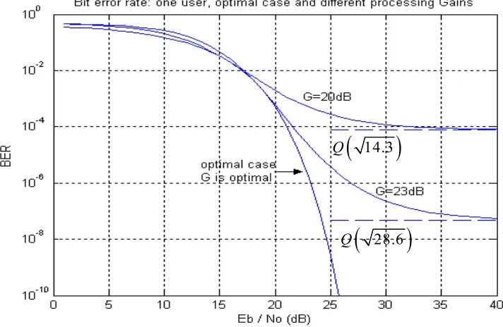
A plot of the BER for the time offset transmitted reference system is shown in Figure 3.7. The BER is plotted as a function of the SNR per bit

0 b E

N for different processing gains (G = 20dB and G = 23dB), and also for the optimal case (G is optimal for each value of

0 b E

N ). It is apparent that for a processing gain equal to 20 dB the bit error rate is minimized by 7.8*10-5, which is equal to the error-floor. The error floor is mainly due the contribution of the noise carrier-noise carrier cross talk. Since the noise carrier-noise carrier cross talk are present even when the AWGN amplitude is zero, bit error rate saturates at large

0 b E

(

)

error-floor

100

Q Q Q 14.3

7 7

G

P = _ _= _ _=

    (3-53)

Figure 3.7 also illustrates that by increasing the processing gain; we can reach lower bit error for high values of

0 b E

N . This is conforming to expression (3-52). At high values of ₀ b E

N the first term in equation (3-52) dominates the other terms and because this term is inversely proportional the processing gain G the BER will be improved.

We can see from Figure 3.7 that for a fixed processing gain G, the BER curve is always above the curve of the optimal BER except for one point where G is optimum. The optimal processing gain G is mainly due the trade of between the noise carrier-noise carrier interferences and the contribution of the AWGN in the information signal. Figure 3.8 shows the BER as a function of the processing gain G for a fixed value of

0 b E

N . We can see that the BER decrease for a while and then reached its minimum at unique value of the processing gain G and then starts increasing as the G increases. Hence for a given value of

0 b E

N the processing gain G should be as close to the to the optimal processing gain as possible to get the low bit error rate.

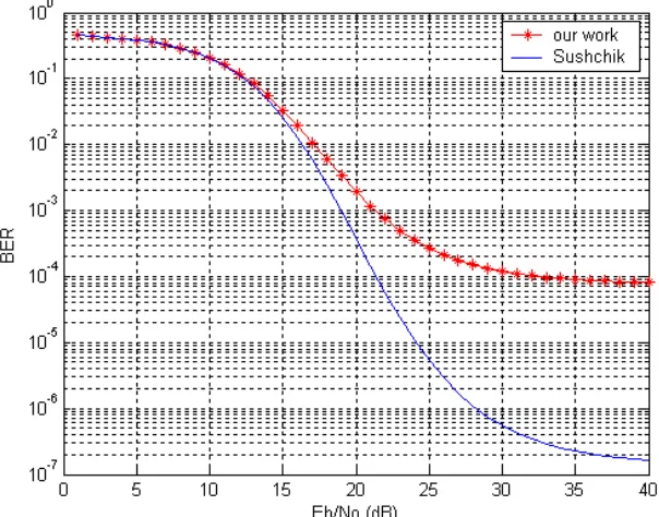
Figure 3.9 compares between our analytical results and those of Sushchik [10]. We can see that Sushchik model has a better link performance than our model. This is due to the kind of the noise carrier used in the two schemes. We used a noise carrier having a Gaussian distribution. But Sushchik used a chaotic carrier having a uniform distribution. A disadvantage of Chaotic signals with uniform distribution is that are difficult to generate.

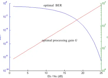
We proved that for a given SNR per bit 0 b E

N , the signal-to-beat noise ratio is optimal only for one value of the processing gain. Thus if equation (3-49) is fulfilled, the optimal bit error rate will be equal to:

optimal

0 1

Q .

4 2 7 b E P

N

 

= _ _

+

Figure 3.10 shows the BER for the optimal bit error rate (left). The BER is optimal for each value of

0 b E

N . This is due mainly to the trade off between the different contributions of the noise carrier interferences and the contributions of the AWGN interferences in the information band for different processing gains. Figure 3.10 also shows the optimal processing gain G as a function of

0 b E

N (right). The optimal processing gain is a linear function of ₀ b E

N . It implies that the processing gain can be adaptively optimised to different values of

0 b E

N to get the lower BER. This is undesirable because it will increase the complexity of the system.

Figure 3.7:The BER as a function of Eb/No and for different processing gains (G=20dB, G=23 dB), and for the

optimal bit error rate (G is optimal for each value of the SNR per bit Eb/No)

(

14.3

)

Q

(

28.6

)

Figure 3.8: The bit error rate as a function of the processing gain G at a fixed value of Eb/No

Figure 3.9: The BER, our model and Sushchik’s model

0

18

b

E N =

0

20

b

Figure 3.10: The optimum BER as a function of Eb/No (left)

and the corresponding optimum processing gain G (right)

optimal BER

4 Link performance for multiple users

In chapter 3 we investigated the link performance for one transmitter and one receiver. In practice multiple users transmit and receive at the same time. In this chapter we will determine the link performance of the time offset transmitted reference system if there are multiple transmitters and multiple receivers. The last section will study an example in detail.

4.1 Mixer output

4.1.1 Instantaneous mixer output

Figure 4.1 illustrates the time offset transmitted reference system when multiple users transmit at the same time. We will assume that the number of users is equal to M.

Figure 4.1: The time offset transmitted reference system with multiple transmitter and receivers

We denote the signal transmitted by transmitter j by:

( ) ( ) . ( )

j j j j j

y t =x t +m x t−τ (4-1)

( ) j

y t The transmitted signal by transmitter j.

1( ) m t

( )

r

m t

( )

M

m t

+

0

b

T

∫

v1,i

0

b

T

∫

vr i,

0

b

T

∫

vM i,

. . .

. . .

. . .

. . .

1

τ

r τ

M τ

( )

y t

( )

y t

( )

y t

1( ) w t

( )

r

w t

( )

M

w t

1( ) z t

( )

r

z t

( )

M

z t

1( ) x t

( )

r

x t

( )

M

x t

1

τ

r τ

M τ +

+

+ _Χ

Χ Χ

( )

n t

Mod Mod Mod

( )

H f

( )

H f

( )

j

m Information signal transmitted by transmitter j. j

τ The time offset used by transmitter j, which is unique for each transmitter. ( )

j

x t The noise carrier used by transmitter j.

We assume that the noise carriers are mutually independent, and all of them have a Gaussian distribution with a mean value equal to zero. Each receiver receives all transmitted signals corrupted by AWGN. Therefore the input of each receiver can be written as:

1

( ) M _j( ) ( )

j

y t y t n t

=

=

∑

+ (4-2)

( )

n t The Additive White Gaussian Noise process having a mean value equal to zero and having a double sided spectral density

2

0

N

W / Hz. M The number of users transmitting at the same time By writing out yj(t) we get:

1

( ) M _j( ) _j. (_{j j}) ( )

j

y t x t m x t τ n t

=

 

=

∑

_