STATISTICAL ANALYSIS OF THE MARIANA TRENCH GEOMORPHOLOGY USING
R PROGRAMMING LANGUAGE
Polina LEMENKOVA
1,*1 College of Marine Geoscience, Ocean University of China, Qingdao, China
*Correspondence: [email protected] , [email protected]
Abstract. This paper introduces an application of R programming language for geostatistical data processing with a case study of the Mariana Trench, Pacific Ocean. The formation of the Mariana Trench, the deepest among all hadal oceanic depth trenches, is caused by complex and diverse geomorphic factors affecting its development. Mariana Trench crosses four tectonic plates: Mariana, Caroline, Pacific and Philippine. The impact of the geographic location and geological factors on its geomorphology has been studied by methods of statistical analysis and data visualization using R libraries. The methodology includes following steps. Firstly, vector thematic data were processed in QGIS: tectonics, bathymetry, geomorphology and geology. Secondly, 25 cross-section profiles were drawn across the trench. The length of each profile is 1000-km. The attribute information has been derived from each profile and stored in a table containing coordinates, depths and thematic information. Finally, this table was processed by methods of the statistical analysis on R. The programming codes and graphical results are presented. The results include geospatial comparative analysis and estimated effects of the data distribution by tectonic plates: slope angle, igneous volcanic areas and depths. The innovativeness of this paper consists in a cross-disciplinary approach combining GIS, statistical analysis and R programming.
Keywords: R, statistical analysis, programming, Mariana trench, oceanography, geomorphology
Introduction
The goal of this study is to analyze factors affecting geomorphological structure of the Mariana Trench. Mariana Trench is a long and narrow topographic depression of the seafloor located in the west Pacific ocean, 200 km to the
east of the Mariana Islands, east of the Philippines.
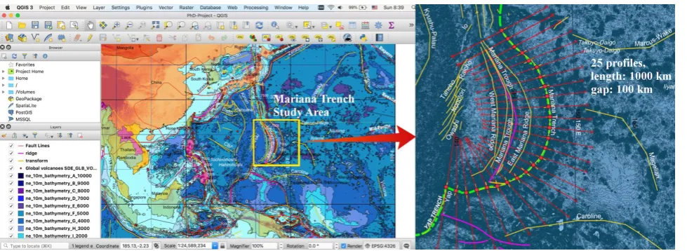
Figure 1. Study area: Mariana Trench. Visualization: QGIS 3.0.
It is known as the deepest part of the ocean floor reaching a maximum-known depth of 10,984±25 m (95%) at 11.329903°N /142.199305°E (Figure 1) at the Challenger Deep (Gardner et al., 2014). It has a distinctive morphological feature of the convergent Pacific plate boundaries, along which lithospheric plates move towards each other. The total length of the trench measures ca. 2,550 km long on average.
1. General characteristics of the Mariana Trench
1.1. Processes of the deep-sea sedimentation
Processes of the deep-sea terrigenous sedimentation are formed by the transfer of the erosion materials from the adjacent land. The main processes include transportation, deposition and re -deposition of the sedimentation materials. The origin of the deep ocean sedimentation is diverse. In general, apart from the sediments from the rivers, the terrigenous material goes to the oceans through iceberg melting and glacial deposits transferred to the seafloor, as well as dusty material moved by the aeolian processes. Normally, the sediments transferred by rivers are deposited within the shelf sublittoral areas, and rarely reach deeper regions of the continental slope and, even less the abyssal basins. However, sediments deposited on the shelf may move to the deeper parts of the ocean includi ng hadal trenches, due to further move from the shelf edge downwards, avalanche sedimentation, i.e. gravitational flows, which are caused by the gravity. For the case of the Mariana Trench, the deep currents flow through the trench ventilating its bottom water flowing through the West Pacific trenches originates from the Southern Ocean and flows northward (Warren et al., 1988), in a clockwise direction, passing through the trenches on the west of the Pacific (i.e. the Kermadec Trench and the Tonga Trench. Through the Samoan Passage, it flows northwest across the equator to the east Mariana Trench. Among other hadal trenches, Mariana Trench is the largest structural traps located in the continental margins. It stretches for hundreds kilometers and has a narro w depression on the ocean floor with very steep slopes and the depths of 3-5 km width of the bottoms rarely exceeding 5 km in breadth (Nakanishi et al., 2011).
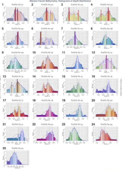
Figure 4. Histograms of the 25 profiles, Mariana Trench. Visualization: R.
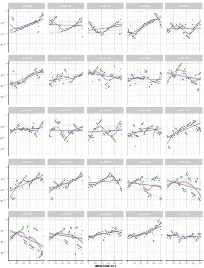
Figure 5. Regression analysis of the 25 profiles, Mariana Trench. Visualization: R.
1.2. Bathymetry and the system of crack
Mariana Trench presents a strongly elongated, arched in plan and lesser rectilinear depression. Its transverse profile is asymmetric: the slope is higher on the side of the Mariana island arc. The slopes of the trench are dissected by deep underwater canyons. Various narrow steps are also often found on the slopes of the trench. On the longitudinal profiles of the bottom of the Mariana there are many deepwater detected transverse steps and thresholds connected by the movements of the earth's crust along transverse faults (Zhou et al., 2015).
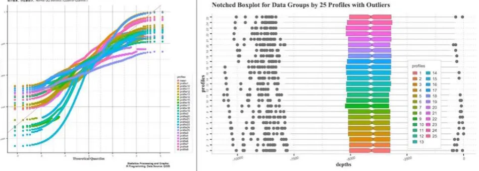
Figure 6 Quantile statistics (QQ), empirical cumulative density function (ECDF) and notched plot
These thresholds can play important role in the evolution of the deep water trough, for example, to control the intensity of its filling by sedimental precipitation. In this process very important are the streams of the precipitation moving along the bottom from the part of the trough which is closer to the continent (Taira et al., 2004). At the bottom of the trough there is a transverse threshold, which can present kind of a dam, in front of which there is accumulation of a thick layer of sediment precipitation.
Figure 7. Distribution of slope angle, sedimental thickness, depth and igneous volcanic zones, by four tectonic plates
as subjects to the gravitational flow system of the submarine canyons and valleys (Kawabe, 1993). Complex distribution of the various geomorphic material on the adjacent abyssal plains of the ocean contributes to the formation of the geomorphic features of the particular region of the Mariana Trench.
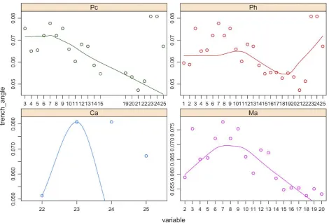
Figure 8. Multiple panel by groups: four tectonic plates, trench slope angle in the deepest point
1.3. Igneous volcanic areas
Mariana Trench is an important integral feature of the active continental margins that naturally includes deep plate subduction. Subduction of slabs of oceanic lithosphere into the deep mantle involves a wide range of the geophysical and geochemical processes and is of major importance for the physical and chemical evolution of the Earth (Miller et al., 2004). Thus, the subduction and subduction-related volcanism are the major processes through which geochemical components are being recycled between the Earth’s crust, lithosphere and mantle (Yoshioka et al., 2015). A large proportion of the world’s earthquakes and volcanoes are related to the subduction (Kirby et al., 1996). Deep sea volcanism results from a range of processes including dehydration, melting and melt migration. The deepest known earthquakes occur in the subducted lithosphere at depths of 660–700 km but their cause is still not explained. In addition, the motion and velocities of the lithospheric plates at the Earth’s surface are controlled largely by the buoyancy forces that drive subduction. Because of the wide variety of processes involved, subduction zones can be regarded as natural laboratories through which dynamic behaviour in the Earth’s mantle can be studied.
Factors affecting plate subduction include hydrothermal factors (Yoshikawa et al., 2012), buoyancy forces, rheology of mantle minerals, stabilities of hydrous minerals, partial melting, mechanisms and rates of melt migration, kinetics of phase transformations, mechanisms of deep earthquakes, geochemical recycling, and the processes of continental collision that result from subduction (Miller et al., 2005). One fundamental problem concerns the depth to which subducted lithosphere penetrates into the mantle because this is related to the scale of mantle convection and the Earth’s evolution.
1.4. Seafloor spreading
Figure 9. Multiple panel by groups: four tectonic plates, depth scope (min-max) by profiles using overlapping points
The Japanese Lineation set is a Mesozoic magnetic anomaly lineation, it exists in the East Mariana Basin, east of the Mariana Trench (Nakanishi et al., 1992), which means that the subducting plate along the southern part of the Mariana Trench is a part of the Pacific plate formed in the Mesozoic. Other remarkable topographic feature of the Mariana Trench includes a set of many elongated ridges and escarpments accompanied by the plate bending on the outer slopes with two existing distinct strikes for these structures. The elongated structures have two strikes: N85°E and the same as the trench axis; N70°E. Most bending-related structures except those near the trench axis, were formed by the reactivation of the seafloor spreading fabric.
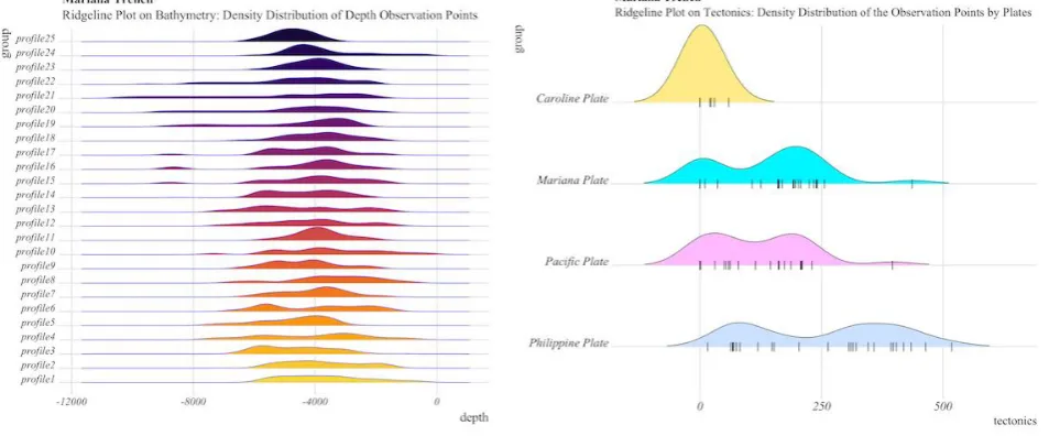
Figure 10. Ridgeline Plots by tectonic plates and bathymetric profiles
The presence of cracks is another distinguished geological feature of the Mariana Trench (Ogawa et al., 1997). Mariana Trench has many open prominent cracks on its surface, up to a few meters deep and a few hundred meters long on the diatomaceous clayey sediment surfaces of its oceanward slopes. The shape of the cross-section is Y-shaped. More precisely, the bottom is a very narrow (1-3 km), yet in some places wide (several tens of kilometers) flattened.
2. Methods and procedures
The methodological scheme includes four general steps of the statistical analysis of the morphology of the Mariana Trench:
2. Statistical analysis of data distribution: calculation and visualisation for regression analysis, histograms, boxplots with outliers, theoretical and sample quantiles (QQ);
3. Comparative geospatial analysis by four tectonic plates: categorywise compositional bar charts on the depths distribution in observation points; multi-dimensional strip plots by four tectonic plates on maximal depth values, slope angle steepness, closeness of the igneous volcanic zones and thickness of the sediment layer; 4. Clustering (by k-means method), correlation ellipses, data partition, grouping and sorting.
Here the geospatial analysis aims to extract a more regular impact factors of the geologic morphology development; whereas the cluster analysis and computing correlation matrices extracts the groups and classes in a total cloud of observation points. Statistical analysis has been performed by means of R (Borradaile, 2003). The R scripting is composed of separate written codes and an algorithm for data processing.
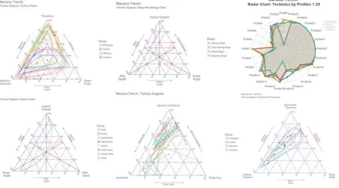
Figure 11. Ternary diagrams and radar chart: facetted plot
The R codes presented below generate a call for various statistical formulae and algorithms used by the machine for the data processing.
2.1. Data collection for the GIS project
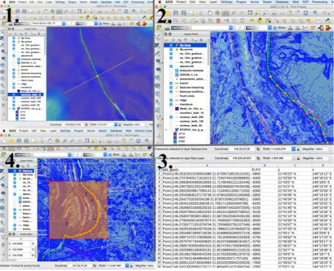
The GIS part of the research is performed in the QGIS (Figure 1). Using QGIS plugins several complex tasks were separated into smaller and more manageable components (e.g. reading coordinates, crossing profile lines, etc). Various geospatial data have been uploaded into the GIS to form the GIS project: bathymetric features of the trench, sediment thickness, location of igneous volcanic zones, distribution of the tectonic plates, etc. The GIS project has been projected into the UTM cartesian coordinate system (square N-55). The GIS processing part consisted in following steps. Firstly, 25 1000-km long cross-section bathymetric profiles were digitized across the trench, as illustrated on Figure 2. The geometry of the first of the 25 profiles has been digitized across the Mariana Trench manually. Then, the line has been copied and re-entered for the next 24 profiles with a distance between every two neighbour lines of 100 km. The numbering of the profiles goes consequently from the north to the south, from Nr. 1 to Nr. 25, respectively. Hence, every profile contained 518 measurement points, XY coordinates, elevation depth data and thematic geological data (e.g. thickness of the sediment layer) stored in an attribute table. The QGIS tool plugin “Lat Lon Tools” adding projected coordinated has been installed to activate QGIS option of adding x and y values directly to the Spreadsheet. The total dataset comprises of large amount of 12950 observations. The data were then copied into a table which was used further in this work for the statistical processing. The created profiles are visualized on Figure 3.
2.2. Analysis of Data Distribution
Figure 12. Category-wise distribution of depth by tectonic plates (left); circular bar plot, arranged by depth (right)
2.2.1. Histograms
The histogram plots (Figure 4) show normal distribution of the depth observation data by the bathymetric cross-section profiles, as well as their outliers, skewness, median, mean, average, maximal, minimal and quartile distribution values. For each of 25 bathymetric profile various colours are taken for the following statistical data of depth values along the profile: ‘black’ curves stands for normal distribution, ‘blue’ curves – for density distribution. Vertical dashed lines: ‘purple’ – median values, ‘green’ – mean values. The histograms have been drawn using R library{ggplot2}. On the first step a single histogram for each of bathymetric 25 profiles was created.
The full R script to create one histogram is as follows (here: for the profile Nr. 1, further applied for every one from 25 profilesby changing the name of the file from ‘01’ to ‘02’, and so on to ‘25’):
MDepths <- read.csv("Depths.csv", header=TRUE) X01<- MDepths[,01]
X01<-X01[!is.na(X01)] as.data.frame(X01) dat01<- data.frame(X01) p01<-ggplot(dat01, aes(X01)) +
labs(title = "Profile Nr.01", x = "Depths, m", y = "Density") + theme(
plot.title = element_text(family = "Skia", face = 2, size = 10), panel.background=ggplot2::element_rect(fill = "gray91"),
legend.position = c(.95, .95),legend.justification = c("right", "top"), legend.box.just = "right",
legend.margin = margin(6, 6, 6, 6),legend.direction = "vertical", legend.background = element_blank(), legend.key.width = unit(.5,"cm"),legend.key.height = unit(.3,"cm"),legend.spacing = unit(.3,"cm"), legend.box.background = element_rect(colour = "honeydew4",size=0.2),
legend.text = element_text(family = "Arial", colour="black", size=6, face=1),legend.title = element_blank(), strip.text.x = element_text(colour = "white"),
panel.grid.major = element_line("white", size = 0.3),
panel.grid.minor = element_line("white", size = 0.3, linetype = "dotted"),
axis.text.x = element_text(family = "Arial", face = 3, color = "gray24",size = 5, angle = 0), axis.text.y = element_text(family = "Arial", face = 3, color = "gray24",size = 4, angle = 90), axis.ticks.length=unit(.1,"cm"),axis.line = element_blank(),
axis.title.y = element_text(margin = margin(t = 20, r = .3), family = "Times New Roman", face = 1, size = 6), axis.title.x = element_text(family = "Times New Roman", face = 1, size = 6,margin = margin(t = .2))) +
scale_x_continuous(breaks = pretty(dat01$X01, n = 4), minor_breaks = seq(min(dat01$X01), max(dat01$X01), by = 500)) + scale_y_continuous(breaks = scales::pretty_breaks(n = 4),labels = scales :: percent) +
scale_fill_distiller(palette = "RdGy") +
scale_color_manual(name = "Statistics:", values = c(median = "purple", mean = "green4",density = "blue", norm_dist = "black")) +
stat_function(fun = dnorm, args = list(mean = mean(dat01$X01), sd = sd(dat01$X01)), lwd = 0.2, color = 'black') + stat_density(
geom = "line", size = .3, aes(color = "density")) +
geom_vline(aes(color = "mean", xintercept = mean(X01)), lty = 4, size = .3) + geom_vline(aes(color = "median", xintercept = median(X01)), lty = 2, size = .3) + geom_vline(aes(color = "norm_dist", xintercept = dnorm(X01)), lty = 2, size = .3)
Using this script further 25 profiles have been created, consequently, p01, p02, … p25.
On the next step the combination of 25 profiles on one layout (Figure 4) has been done using following R script: library(cowplot)
figure <-plot_grid(
p01 + theme(legend.position="none"), p02 + theme(legend.position="none"), # continue sequently until profile Nr. 25: p25 + theme(legend.position="none"),
labels = c("1", "2", "3", "4", "5", "6", "7", "8", "9", "10", "11", "12", "13", "14", "15", "16", "17", "18", "19", "20", "21", "22", "23", "24", "25"),
ncol = 4, nrow = 7)
On the final step the annotation for the figure has been created using following R script: figure_all_cowplot<- annotate_figure(figure,
top = text_grob("Mariana Trench Bathymetry: Histograms of Depth Distribution", color = "lightsteelblue4", face = "bold", size = 10),
bottom = text_grob("Data processing: \n R, QGIS", color = "blue", hjust = 1, x = 1, face = "italic", size = 8), left = text_grob("Figure arranged using R, ggpubr", color = "slategray4", size = 8, rot = 90),
right = text_grob("1000-km length profiles", color = "slategray4", size = 8, rot = 270), fig.lab = "Profiles 1-25", fig.lab.face = "bold", fig.lab.size = 8, fig.lab.pos = "bottom.left")
ggsave("figure_all_cowplot.pdf", device = cairo_pdf, fallback_resolution = 300, width = 210, height = 297, units = "mm")
Generated plot of te 25 histograms (Figure 4) illustrates the frequency of the score occurrences in a continuous data set of the bathymetric depths that has been divided into classes showing variation in the samples of the depths, assumptions of the underlying statistical distribution of observation points values.
2.2.2. Regression Analysis
To estimate the relationships between variables a regression analysis has been done using existing methods (Journel, 2000). Regression analysis and facetted plot wrapping for 25 bathymetric profiles were executed by R library {ggplot2}. Using non-parametric regression analysis the conditional expectation of the dependent variable (that is depth values) given the independent variables was estimated (Figure 5). The confidence interval for each of 25 profiles has been done by four methods, visualized by the facetted plot wrapping for the series data comparison.
The regression analysis reveals how the typical value of the criterion variable changes when any one of the independent variables change, while the other independent variables are fixed. The formula describing regression equation describing the relationship between two variables used in this research is as follows:
Y = a + bX + e(1)
The literature refers (Journel, 2000) to three major applications of the regression analysis including general loess method (“glm”), loess method (“lm”) and loess method (“loess”), all of which were tested in this research.
The following R codes were used for the four methods of the regression analysis visualized on Figure 5: Loess_profile11 <- ggplot(MDF, aes(x = observ, y = profile11)) +
geom_point(aes(x = observ, y = profile11, colour = "Samples", shape = "Samples"), show.legend=TRUE) +
geom_smooth(aes(x = observ, y = profile11, colour = "Loess method"), method = loess, se = TRUE, span = .4, size=.3, linetype = "solid", show.legend=TRUE) +
geom_smooth(aes(x = observ, y = profile11, colour = "Glm method"), method = glm, se = FALSE, span = .4, size=.4, linetype = "dotted", show.legend=TRUE) +
geom_smooth(aes(x = observ, y = profile11, colour = "Lm method"), method = lm, se = TRUE, size=.3, linetype = "solid", show.legend=TRUE) +
geom_quantile(aes(x = observ, y = profile11, colour = "Quantiles"), linetype = "solid", show.legend=TRUE) + xlab("Observations") +
ylab("Depths, m") +
scale_shape_manual(values = c("Samples" = 1)) + # shape of the point (here: Nr1 – "transparent circle") labs(title="Mariana Trench, Profile 11.",
subtitle = "Local Polynomial Regression, \nConfidence Interval, Quantiles \n(LOESS method: locally weighted scatterplot \nsmoothing for non-parametric regression)", caption = "Statistics Processing and Graphs: \nR Programming. Data Source: QGIS") + theme()
Figure 13. Double-Y-axis plot of correlation of environmental factors
The quantiles were drawn by calling geom_quantile function of R. The generalized linear models (glm method) was used to give a symbolic description of the linear predictor of depth variability within each bathymetric profile, and a description of the error distribution in a range of the depth observation points. The quantiles graphically depict groups of the depth values through their distribution mode, according to the methods of the descriptive statistics. The spacings between the different parts of the box indicate the degree of the dispersion, i.e. spread, and skewness in the bathymetric data, and show outliers. The data outside the upper and lower quartiles are the outliers that are plotted as individual points. The outliers are the non-usual values of the depths indicating specific features of the geomorphology with extra deep values. The histograms show probability of the density distribution of the bathymetric observation by the profiles, i.e. how likely is that the data will belong to this or that part of the group values within certain depth range.
2.2.3. Notched Boxplots
The notched boxplot (Figure 6) showing distribution of the depths with majority of the data from -3000 to -5000 m and outliers (the deepest points) show that from profile 1 to 16 the general depth increase with deepest values at profiles 10 and 11. The R code for generating notched boxplot is as follows:
#Part 1
# step-2. Cleaning dataframe from the от NA values MDepths_df <- na.omit(MDepths)
row.has.na <- apply(MDepths_df, 1, function(x){any(is.na(x))}) # check up the NA sum(row.has.na) # sup up theNA, result: [1] 0
head(MDepths_df) # look up dataframe
# Part 2: generating whisker boxplot using dataframe MDepths_df. # step-3. Adding palette, lines type, Chinese fonts.
p<- ggboxplot( MDepths_df,
title="马里亚纳海沟。剖面11。Mariana Trench, Profiles 1-25.",
subtitle = "统计图表。箱形图。Notched Boxplot for Data Groups by 25 Profiles with Outliers)", caption = "Statistics Processing and Graphs: \nR Programming. Data Source: QGIS",
x = "profiles", y = "depths", width = 0.8, notch = TRUE, fill = "profiles", linetype = 1, size = .1, outlier.colour = "grey44", palette = c("magma"), orientation = "horizontal")
# step-4. Adding theme and palette using default format boxplot_Mariana<- p + theme()
As can be seen from the notched boxplot (Figure 6), the shallowest parts of the trench are located in the profiles 24 and 25 where Mariana Trench crosses the Yap Trench, the oceanic trench near Yap Island in the western Pacific Ocean.
2.3. Comparative Geospatial Analysis by Four Tectonic Plates
Mariana Trench crosses four tectonic plates: Mariana, Philippine, Pacific and Caroline. Therefore, a comparative analysis of multidimensional data was performed to analyse inter-relationships between the geographic location of the specific parts of the trench and factors that may impact changes in the geomorphic systems. Using existing methodology (Bretz et al., 2011), various dependences between the impact factors were tested in the current research by various approaches of the comparative analysis: Figures 7, 8 and 9.
First, the distribution of various environmental factors affecting the morphology of the trench were analysed: slope angle, sedimental thickness, depth and closeness of the igneous volcanic zones to the selected bathymetric profiles (Figure 7).
Second, the changes in the trench deepest angle, calculated as tg(A/H), where A is the width, and H is the maximal depth of the profile, were calculated for each of the 25 bathymetric profiles and compared, respectively (Figure 8).
Figure 14. Results of the k-means of the clustering of the Mariana Trench profiles
2.3.1. Pairwise Comparison Using Series of Multiple Strip Plots Divided by Groups
The multiple panel strip plots were generated in a combined plot using {LatticeExtra2} package of R by stripplot function. The distribution of the slope angle, sediment thickness, depth and closeness of the igneous volcanic zones towards Mariana Trench, by four tectonic plates is shown on Figure 7. The R code used is as follows:
# Part-1. Create data frame
# step-1. Read in data table. Generate data frame. Clean data frame from the NA values MDepths <- read.csv("Morphology.csv", header=TRUE, sep = ",")
MDF <- na.omit(MDepths)
row.has.na <- apply(MDF, 1, function(x){any(is.na(x))}) sum(row.has.na)
head(MDF)
# step-2. merge 4 columns with tectonic plates into one named "tectonic plates" MDFt = melt(setDT(MDF), measure = patterns("^plate"), value.name = c("tectonic plates")) head(MDFt)
# step-3. Make column with tectonic plates as factor value (variable) MDFt$variable =as.factor(MDFt$variable)
levels(MDFt$variable)=c("Philippine", "Pacific", "Mariana", "Caroline") # explicitly rename 4 tectonic plates to be shown as names on X axis (otherwise they will be shown as numbers)
# Part-2. Create structured namе (Title + Subtitle by various fonts) in {LatticeExtra} using doubleTitle function library(latticeExtra)
# step-4.
doubleTitle <- function(a,b) { gTree(children=gList(
textGrob(a, gp=gpar(fontsize=10, fontface=1), y=0, vp=viewport(layout.pos.row=1, layout.pos.col=1)), textGrob(b, gp=gpar(fontsize=8, fontface=3), y=0, vp=viewport(layout.pos.row=2, layout.pos.col=1))
), vp=viewport(layout=grid.layout(nrow=2, ncol=1)), cl="doubletitle") }
heightDetails.doubletitle <- function(x, recording=T) {
Reduce(`+`, lapply(x$children, grid:::heightDetails.text)) * 2 }
# Part-3. Strip Plot
# step-5. Generate strip plots (vertical division of the data by four categories, here: 4 tectonic plates) # variant 5.1 bathymetry (steepness of the slope angles):
s1<- stripplot(slope_angle ~ variable, data = MDFt, jitter.data = TRUE, pch = 20, palette="Set2", xlab = list(label="Tectonic Plates", cex= 0.60),
ylab = list(label="Slope Angle(tg(A/H))", cex= 0.60),
main=doubleTitle("Mariana Trench","Slope Angle(tg(A/H)) in 25 Profiles by Tectonic Plates")) s1
# variant 5.2 sedimentation (seabed sediments):
s2<- stripplot(sedim_thick ~ variable, data = MDFt, jitter.data = TRUE, pch = 20, xlab = list(label="Tectonic Plates", cex= 0.60),
ylab = list(label="Sediment Thickness", cex= 0.60),
main=doubleTitle("Mariana Trench","Sediment Thickness in 25 Profiles by Tectonic Plates")) s2
# variant 5.3 bathymetry (minimal depths):
s3<- stripplot(Min ~ variable, data = MDFt, jitter.data = TRUE, pch = 20, xlab = list(label="Tectonic Plates", cex= 0.60),
ylab = list(label="Maximal Depth", cex= 0.60),
main=doubleTitle("Mariana Trench","Maximal Depth in 25 Profiles by Tectonic Plates")) s3
# variant 5.4 geology (igneous volcanic zones):
s4<- stripplot(igneous_volc ~ variable, data = MDFt, jitter.data = TRUE, pch = 20, xlab = list(label="Tectonic Plates", cex=0.60),
ylab = list(label="Igneous Volcanic Areas", cex= 0.60),
main=doubleTitle("Mariana Trench","Igneous Volcanic Zones Distribution in 25 Profiles by Tectonic Plates")) s4
# step-6. merge all four categories on one plot
l <- as_ggplot(g) +
draw_plot_label(label = c("A", "B", "C", "D"), size = 10, x = c(0, 0.5, 0, 0.5), y = c(1, 1, 0.5, 0.5))
2.3.2. Multiple Panels, Divided by Categories
The variation of the slope angle in the deepest point and depths by 25 bathymetric profiles of the Mariana Trench according to four tectonic plates that is crosses is illustrated on Figure 8 and Figure 9. The plots have been created using R code in 4 steps:
# step-1. Creating data frame in R from the initial table (.csv) MDepths <- read.csv("DepthTect.csv", header=TRUE, sep = ",") MDFl <- na.omit(MDepths) # delete possible NA values
row.has.na <- apply(MDFl, 1, function(x){any(is.na(x))}) # check up NA values sum(row.has.na) # sum up NA values, receive: [1] 0
head(MDFl) # look up data frame.
# step-2. Merge category groups by classes (here: tectonics, depths, angles)
DFDT = melt(setDT(MDFl), measure = patterns("^profile", "^tectonics", "^tg"), value.name = c("depth", "tectonics", "trench_angle"))
head(DFDT)
# step-3. Multiple panels by groups: y ~ x | group generate multi-plot
p<- xyplot(depth ~ variable | tectonics, group = tectonics, data = DFDT, type = c("p", "smooth"), scales = "free", main="Multiple ScatterPlot: Depths Distribution by Tectonic Plates", xlab="Profiles, Nr")
# step-4. Generate two variants of the multiple panels by groups: for slope angles and depths
stripplot(trench_angle ~ variable | tectonics, data = DFDT, layout = c(4, 1), jitter.data = TRUE, xlab = "tectonic.plates", ylab = "trench_angle")
stripplot(depth ~ variable | tectonics, data = DFDT, layout = c(4, 1), jitter.data = TRUE, xlab = "tectonic.plates", ylab = "depth")
The resulting graphs show variation of the slope angle in the deepest point (Figure 8) and depths (Figure 9) by 25 bathymetric profiles of the Mariana Trench by four tectonic plates: Mariana, Caroline, Pacific and Philippine.
2.3.3. Ridgeline Plots
The ridge plots (Figure 10) were created to combine information about statistical data on 25 bathymetric profiles: arithmetic density distribution, mean and standard deviation along the profiles in a facetted way. They have lines extending horizontally from the boxes indicating variability of the Mariana Trench depths distribution across all the profiles. The code generated using {ggridges} and {ggplot2} libraries is as follows:
# Part-1 for 4 tectonic plates (Figure 10, right)
# step-1. Read-in initial table. Generate data frame. MDF <- read.csv("Morphology.csv", header=TRUE, sep = ",") MDF <- na.omit(MDF)
row.has.na <- apply(MDF, 1, function(x){any(is.na(x))}) sum(row.has.na)
head(MDF)
# step-2. Merge columns by categories (here: tectonics, 4 plates)
MDTt = melt(setDT(MDF), measure = patterns("^plate"), value.name = c("tectonics")) head(MDTt)
levels(MDTt$variable) = c("Philippine Plate", "Pacific Plate", "Mariana Plate", "Caroline Plate") head(MDTt)
# step-3. Create short data frame only from 2 necessary categories: names of the 4 plates and values of the observation points:
dat <- data.frame(group = MDTt$variable, pweight = MDTt$tectonics, tectonics = MDTt$tectonics)
# step-4. Generate ridgeline plot:
ggplot(dat, aes(x = tectonics, y = group, fill = group)) +
geom_density_ridges(scale = .95, jittered_points=TRUE, rel_min_height = .01, point_shape = "|", point_size = 3, size = 0.25,
position = position_points_jitter(height = 0)) +
scale_fill_manual(values = c("lightsteelblue1", "plum1", "turquoise1", "lightgoldenrod1")) + theme_ridges() +
theme(legend.position = "none",
plot.subtitle = element_text(family = "Times New Roman", face = 1, size = 12), axis.title.y = element_text(family = "Times New Roman", face = 1, size = 12), axis.title.x = element_text(family = "Times New Roman", face = 1, size = 12), axis.text.x = element_text(family = "Times New Roman", face = 3, size = 12), axis.text.y = element_text(family = "Times New Roman", face = 3, size = 12)) + labs(title = 'Mariana Trench',
subtitle = 'Ridgeline Plot on Tectonics: Density Distribution of the Observation Points by Plates') # Part 2: for bathymetric depths (Figure 10, left)
dat <- data.frame(group = MDDl$variable, pweight = MDDl$depth, depth = MDDl$depth) # step-5. Create ridgelines for bathymetry
ggplot(dat, aes(x = depth, y = group, fill = group)) +
geom_density_ridges(scale = 0.95, jittered_points=FALSE, color = "blue", size = 0.2) + labs(title = 'Mariana Trench',
subtitle = 'Ridgeline Plot on Bathymetry: Density Distribution of Depth Observation Points') + scale_fill_viridis(discrete = T, option = "B", direction = -1, begin = .1, end = .9)+
theme_ridges() + theme()
Figure 16. Classification of the k-means clustering of the Mariana Trench by tectonic plates
2.3.4. Categorywise bar plots
To create categorywise plot (Figure 11, left) following methodology was used. First, the table was read into R: MDepths <- read.csv("DepthTect.csv", header=TRUE, sep = ",")
MDF <- na.omit(MDepths)
row.has.na <- apply(MDF, 1, function(x){any(is.na(x))}) sum(row.has.na) head(MDF)
DFDT = melt(setDT(MDF), measure = patterns("^profile", "^tectonics", "^tg"), value.name = c("depths", "tectonics", "angles"))
Third, the plot function was called by the following code using created data frame in the previous step: g <- ggplot(DFDT, aes(variable)) + geom_bar(aes(fill = tectonics), width = 0.5, na.rm = TRUE) + theme(axis.text.x = element_text(angle=65, vjust=0.6)) +
xlab("Profiles, Nr.") + ylab("Observation Points") + labs(title="马里亚纳海沟。剖面1-25。Mariana Trench, Profiles Nr.1-25.",
subtitle = "统计图表。地貌聚类分析, 条形图。Categorywise Bar Chart.
\nDistribution of Observation Points across Tectonic Plates: \nMariana, Philippine, Pacific and Caroline", caption = "Statistics Processing and Graphs: R Programming. Data Source: QGIS") + scale_fill_brewer(palette = "RdBu") + theme()
To create circular barplot divided by groups the following full R code was used by :library{tidyverse}. Here: start from the step 3 after the fist two steps of creating the data frame to avoid repetition:
# step-3 create short data frame from 3values (here: value – the length of the petal of the circle) data<- data.frame(
id = MDFt$profile, # profile numbers as factor value, i.e. repetition 1:25 individual = paste("Profile", seq(1,25), sep=""),
group = MDFt$variable, # here: 4 tectonic plates
value = MDFt$tectonics) # here: value of the sediment thickness layer (the length of the petal circle)
levels(MDFt$variable) = c("Philippine" , "Pacific", "Mariana", "Caroline") # implicitly indicate the names of the platesto write on the axis X
# Order data:
data = data %>% arrange(group, value)
# step-4 create empty bar to add some space at the end of each group while visualizing the plot empty_bar=3
to_add = data.frame( matrix(NA, empty_bar*nlevels(data$group), ncol(data))) colnames(to_add) = colnames(data)
to_add$group=rep(levels(data$group), each=empty_bar) data=rbind(data, to_add)
data=data %>% arrange(group) data$id=seq(1, nrow(data))
# Part-2.
# step-5 create labels and from the name and the y position of each label label_data = data
number_of_bar=nrow(label_data)
# step-6 calculate the angles of the labels
angle = 90 - 360 * (label_data$id-0.5) /number_of_bar # I substract 0.5 because the letter must have the angle of the center of the bars. Not extreme right(1) or extreme left (0)
label_data$hjust<-ifelse(angle < 90, 1, 0) # distribute the labels right-left
label_data$angle<-ifelse(angle < -90, angle+180, angle) # flip angles to make them readable for visualizing purposes # Part-3 Draw circlal barplot
# step-7. prepare a data frame for the base lines base_data=data %>%
group_by(group) %>%
summarize(start=min(id), end=max(id) - empty_bar) %>% rowwise() %>%
mutate(title=mean(c(start, end)))
# step-8. prepare a data frame for the grid (scales) grid_data = base_data
grid_data$end = grid_data$end[ c( nrow(grid_data), 1:nrow(grid_data)-1)] + 1 grid_data$start = grid_data$start - 1
grid_data=grid_data[-1,] # step-9.
p <- ggplot(data, aes(x = as.factor(id), y = value, fill = group)) +
geom_bar(aes(x = as.factor(id), y = value, fill = group), stat="identity", alpha=0.5) + # scale_fill_distiller(palette = "Set1") +
scale_fill_manual(values = c("purple", "deeppink", "blue", "cyan")) +
# step-11: draw small additional lines indicating scales in the empty spaces between the petals here from 25-100, further from 500 over 100.
geom_segment(data=grid_data, aes(x = end, y = 500, xend = start, yend = 500), colour = "grey", alpha=1, size=0.3 , inherit.aes = FALSE ) +
geom_segment(data=grid_data, aes(x = end, y = 400, xend = start, yend = 400), colour = "grey", alpha=1, size=0.3 , inherit.aes = FALSE ) +
geom_segment(data=grid_data, aes(x = end, y = 300, xend = start, yend = 300), colour = "grey", alpha=1, size=0.3 , inherit.aes = FALSE ) +
geom_segment(data=grid_data, aes(x = end, y = 200, xend = start, yend = 200), colour = "grey", alpha=1, size=0.3 , inherit.aes = FALSE ) +
geom_segment(data=grid_data, aes(x = end, y = 100, xend = start, yend = 100), colour = "grey", alpha=1, size=0.3 , inherit.aes = FALSE ) +
geom_segment(data=grid_data, aes(x = end, y = 80, xend = start, yend = 80), colour = "grey", alpha=1, size=0.3 , inherit.aes = FALSE ) +
geom_segment(data=grid_data, aes(x = end, y = 60, xend = start, yend = 60), colour = "grey", alpha=1, size=0.3 , inherit.aes = FALSE ) +
geom_segment(data=grid_data, aes(x = end, y = 40, xend = start, yend = 40), colour = "grey", alpha=1, size=0.3 , inherit.aes = FALSE ) +
geom_segment(data=grid_data, aes(x = end, y = 20, xend = start, yend = 20), colour = "grey", alpha=1, size=0.3 , inherit.aes = FALSE ) +
# step-12. Add scale annotations showing the value of each 100/75/50/25 lines
annotate("text", x = rep(max(data$id),9), y = c(20, 40, 60, 80, 100, 200, 300, 400, 500), label = c("20", "40", "60", "80", "100", "200", "300", "400", "500") , color="grey", size = 2 , angle=0, fontface="bold", hjust=1) +
ylim(-200,550) + # ylim creates 2 diameters of the circle: outer and inner ones.
# step-13: ylim у is 550, because all values for the tectonic plates do not exceed 550 (i.e. outer circle) # here: diameter of the inner circle = 50
+ theme(
legend.position = "none", axis.text = element_blank(), axis.title = element_blank(),
plot.title = element_text(margin = margin(t = 0, r = 0, b = 0, l = 0), size = 10, face = "bold"), plot.margin = unit(rep(-1,4), "cm")
) +
coord_polar() +
geom_text(data = label_data, aes(x = id, y = value+10, label = individual, hjust=hjust), color="black", fontface="bold",alpha=0.6, size=2.0, angle= label_data$angle, inherit.aes = FALSE ) +
# Add base line information
geom_segment(data = base_data, aes(x = start, y = -5, xend = end, yend = -5), colour = "black", alpha=0.8, size=0.6 , inherit.aes = FALSE ) +
geom_text(data = base_data, aes(x = title, y = -18, label = group), hjust=c(1,1,0,0), colour = "black", alpha=0.8, size=3, fontface="bold", inherit.aes = FALSE)
p
2.3.5. Ternary diagrams and Radar chart
Ternary diagrams and Radar chart were plotted (Figure 12) to show the triple correlation of several factors across tectonic plates: slope morphology classes, tectonics, igneous volcanic areas, aspect degree, slope angle, sedimental thickness. The programming R code for the ternary diagrams is as follows:
MT1<- ggtern(data= MDTer,aes(x,y,z,color = Group)) + theme_rgbw() +
geom_point() +
scale_color_manual(values = c("green", "red", "orange", "blue")) + labs(x="Igneous \nVolcanos",y="Tectonics",z="Slope \nAngle", title="Mariana Trench",
subtitle="Ternary Diagram: Tectonic Plates") + geom_Tline(Tintercept=.5,arrow=arrow(), colour='red') + geom_Lline(Lintercept=.2, colour='magenta') +
geom_Rline(Rintercept=.1, colour='blue') + geom_confidence_tern()
The radar chart (Figure 12, upper right) has been generated using following R code by {fmsb} library: #Part 1 Generating data frame
# step-1. Read-in initial table with bathymetic and geomorphological data MDepths <- read.csv("Morphology.csv", header=TRUE, sep = ",")
MDF <- na.omit(MDepths)
row.has.na <- apply(MDF, 1, function(x){any(is.na(x))}) sum(row.has.na)
head(MDF)
# step-2. Merge group categories by classes
MDFt = melt(setDT(MDF), measure = patterns("^plate"), value.name = c("tectonics")) head(MDFt)
levels(MDFt$variable) = c("Philippine" , "Pacific", "Mariana", "Caroline") Plates<- c("Philippine", "Pacific", "Mariana", "Caroline")
# Part-2. Radar Chart. library(fmsb)
set.seed(25)
# step-3. Create mini-set of 2 values.
radardataM =as.data.frame(matrix(MDFt$tectonics, ncol=25, nrow=4)) colnames(radardataM)<- c(paste("Profile", seq(1:25), sep=""))
rownames(radardataM)<- c("Philippine", "Pacific", "Mariana", "Caroline") # step-4. add 2 lines to the dataframe: max-min of each topic radardataM <- rbind(rep(0, 25) , rep(518, 25) , radardataM)
# step-5. The default radar chart proposed by the library: radarchart(radardataM)
# step-6. Custom the radarChart
colors_border=c(rgb(0.2,0.5,0.5,0.9), rgb(0.8,0.2,0.5,0.9), rgb(0.7,0.5,0.1,0.9), rgb(0.2,0.7,0.4,0.9)) colors_in=c(rgb(0.2,0.5,0.5,0.1), rgb(0.8,0.2,0.5,0.1), rgb(0.7,0.5,0.1,0.1), rgb(0.2,0.7,0.4,0.1)) radarchart( radardataM , axistype=1 , #custom polygon
pcol=colors_border , pfcol=colors_in , plwd=4 , plty=1,
cglcol="grey", cglty=1, axislabcol="grey", caxislabels=seq(0,20,5), cglwd=0.8, #custom grid vlcex=0.8 , #custom labels
title ="Mariana Trench. \nRadar Chart: Tectonics by Profiles 1:25", cex=0.7) legend(x=1.2, y=1.0, legend = rownames(radardataM[-c(1,2),]),
bty = "n", pch=20 , col=colors_in , text.col = "grey", cex = 0.8, pt.cex = 2)
2.3.6. Pairwise double-Y-axis
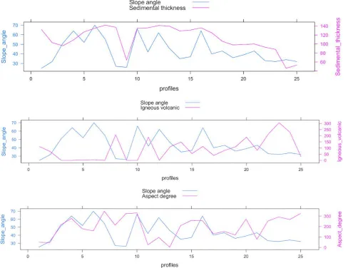
The pairwise double-Y axis (Figure 13) was drawn to analyse the effect of the bi-factor correlation between the slope angle and other variables. The following script runs the model in each case, calculates the X-Y dependences and places both graph on one plot, which his very convenient for comparative studies. The following is a code for the double-Y axis with correlations "Slope angle", "Sedimental thickness" created by library{latticeExtra} in R in 7 steps:
# step-1. Create data set for the new data frame (only 3 necessary values: profiles, slope angle and sediments) set.seed(1)
profiles = MDF$profile
Slope_angle = MDF$slope_angle
Sedimental_thickness = MDF$sedim_thick
data=data.frame(profiles, Slope_angle, Sedimental_thickness) # step-2 plot ‘two in one’ graphs:
p<- xyplot(Slope_angle + Sedimental_thickness ~ profiles, data, type = "l") # step-3. Read-in graphs 1 and 2 into objects
obj1 <- xyplot(Slope_angle ~ profiles, data, type = "l" , lwd=1)
obj2 <- xyplot(Sedimental_thickness ~ profiles, data, type = "l", lwd=1) # step-6. Subscript second axis Y:
doubleYScale(obj1, obj2, add.ylab2 = TRUE) # step-7. Add legend:
Figure 17. Correlation matrix
At the end of each run, the final results are copied to the p1, p2 and p3 plot, and afterwards combined three graphs on one plot. The results of the plotting are shown on the Figure 13.
2.4. Clustering (k-means method), Correlation and Data Grouping
The next working step included finding correlations among the geomorphic factors that impact the morphological formation of the profiles. To this end, cluster analysis and correlation ellipses were created.
2.4.1 Clustering (k-means method) by R library{factoextra}
The k-means clustering, a machine learning technique for classification performs data partition into set up number of clusters, has been done using R library{factoextra}. The goal of the k-means clustering was to perform partition of the dataset of the observations across Mariana Trench into clusters, in which each depth observation belongs to the cluster with the nearest mean, serving as a prototype of the cluster. The performed clustering is sensitive to the initial random selection of the cluster centers. Therefore, several clusters has been tested: starting from 2 to 7. This function provides a solution using a hybrid approach by combining the hierarchical clustering and the k-means methods.
The workflow procedure include following steps:
1. Computed hierarchical clustering and cutting the tree in the k-clusters using R code (provided below); 2. Computed pairwise standard scatter plot of k-means cluster correlation (Figure 14).
3. Computed centres (2 to 7 were tested, in total 6 centres) of each cluster (Figure 15); 5. Created correlation matrix (Figure 16).
6. Created groups have been tested according to their distributions by the tectonic plates (Figure 17).
Figure 18. Correlation ellipses and numerical correlation of the factors affecting Mariana Trench geomorphology
The k-means cluster analysis has been done using following R code: # PART 1: create data.frame with geomorphology data
# step-1. Load table, create dataframe
MorDF <- read.csv("Morphology.csv", header=TRUE, sep = ",") head(MorDF)
summary(MorDF) # PART 2: Clustering
# step-2. Create several examples of cluster analysis with various number of cluster centres (k). Here: 5 k2MorDF <- kmeans(MorDF, centers = 5, nstart = 25)
str(k2MorDF) k2MorDF
fviz_cluster(k2MorDF, data = MorDF)
# step-3. Creaing objects for each of the plots (1to 7, here: example for plot 2):
p2 <- fviz_cluster(k2MorDF, geom = "point", data = MorDF) + ggtitle("Nr. of centers k = 2") + theme(plot.title = element_text(size = 10), legend.title = element_text(size=8), legend.text = element_text(colour="black", size = 8))
# step-4. Combine all plots on one layout:
figure <-plot_grid(p2, p3, p4, p5, p6, p7, labels = c("1", "2", "3", "4", "5", "6"), ncol = 2, nrow = 3) # step-5. Add legend, title and theme:
ClustersMariana6 <- figure +
labs(title="马里亚纳海沟。剖面1-25。Mariana Trench, Profiles Nr.1-25.",
subtitle = "统计图表。地貌聚类分析。Geomorphological Cluster Analysis (k-means)", caption = "Statistics Processing and Graphs: \nR Programming. Data Source: QGIS") +
theme(plot.title = element_text(family = "Kai", face = "bold", size = 12),
plot.subtitle = element_text(family = "Hei", face = "bold", size = 10)) # ‘Kai’ and ‘Hei’ fonts indicate Chinese fonts.
Figure 19. Normalized steepness angle (left); level plot of the sedimental thickness (right)
2.4.2 Correlogram Ellipses and Numerical Correlogram
The correlogram ellipses (Figure 18) were generated to visualize correlation between the factors affecting the morphology of the trench. The methodological approach includes calling {ellipse} library and executing following script:
data=cor(MDF)
# step-1Build a Panel of colors by Rcolor Brewer my_colors <- brewer.pal(5, "Spectral")
my_colors=colorRampPalette(my_colors)(100)
# step-2. Order the correlation matrix, to distribute colours by the factors of the values ord <- order(data[1, ])
data_ord = data[ord, ord]
# step-3. variant-1, correlation ellipses:
plotcorr(data_ord , col=my_colors[data_ord*50+50], mar=c(1,1,1,1), outline = TRUE, numbers = FALSE,
main = "Mariana Trench: Correlation Ellipses",
xlab = "Geomorphological, bathymetric and geological factors", ylab = "Geomorphological, bathymetric and geological factors", cex.lab = 0.7)
# step-4. variant-3, numerical correlation:
plotcorr(data_ord , col=my_colors[data_ord*50+50], mar=c(1,1,1,1), outline = TRUE, numbers = TRUE,
main = "Mariana Trench: Numerical Correlation",
xlab = "Geomorphological, bathymetric and geological factors", ylab = "Geomorphological, bathymetric and geological factors", cex.lab = 0.7)
2.4.3 Data Partition
Data grouping and partition has been performed by dividing angles across the trench on to classes (Figure 19, left). The level plot (Figure 19, right) shows the classes on the sedimental thickness across Mariana Trench. The data grouping has been created using libraries {tidyverse} and {ggsignif} for re-ordering and normalization of the steepness angle (Figure 20). In total 5 classes were created that include: strong slope, very strong slope, extreme slope, steep slope, very steep slope. They show classes of the steepness of the trench according to the results of the previously made cluster analysis and correlation matrix. The circular bar plot (Figure 21, left) showing percentage distribution of the sediment thickness according to the slope angle steepnesss by 25 bathymetric profiles has been drawn using R library{tidyverse}. The circulat barplot has been created using following R code using {tidyverse} library:
# Part 1: generate data frame
row.has.na <- apply(MDF, 1, function(x){any(is.na(x))}) sum(row.has.na)
head(MDF)
# Part 2: generate short data frame with 3 values: profiles, sediment thickness and sequence 1:25 library(tidyverse)
data<- data.frame(
id = MDF$profile, # profiles numbers as factor value, here sequence 1:25 individual = paste("Profile", seq(1,25), sep=""),
value = MDF$sedim_thick) # value – length of the circle petal # Part 3 division data into categories
# step-1
Category <- c(paste("Profile", seq(1,25), sep="")) Percent <- MDF$slope_angle
#color = add_transparency(rainbow(length(Percent)), 0.1) may be used for transparency color = rainbow(length(Percent))
# step-2
Category = rev(Category) Percent = rev(Percent) color = rev(color)
# Part 4 generating circle diagram using {circlize} library # step-3
par(mar = c(1, 1, 1, 1)) circos.par("start.degree" = 90)
circos.initialize("a", xlim = c(0, 100)) # 'a` means there is one sector
circos.trackPlotRegion(ylim = c(0.5, length(Percent)+0.5), track.height = 0.8, bg.border = NA, panel.fun = function(x, y) {
xlim = get.cell.meta.data("xlim") # it is c(0, 100) for(i in seq_along(Percent)) {
circos.lines(xlim, c(i, i), col = "#CCCCCC")
circos.rect(0, i - 0.45, Percent[i], i + 0.45, col = color[i], border = "white")
circos.text(xlim[2], i, paste0(Category[i], " - ", Percent[i], "%"), adj = c(1, 0.5), cex = .65)
} })
circos.clear()
text(0, 0, "Mariana Trench \nSlope Angles \nby Profiles 1:25", col = "#CCCCCC", cex = .75)
Created circular diagram is presented on Figure 21, left.
Finally, the logical visualization of the results as Euler-Venn diagram (Figure 21, right) is created as a visual illustration of the most notable geomorphological parameters which enables to analyze correlations between the environmental factors affecting trench geomorphology. The R code for generating Euler-Venn diagram using {venn} library is as follows:
# Part 1. generating data frame:
MDepths <- read.csv("Morphology.csv", header=TRUE, sep = ",") MDF <- na.omit(MDepths)
row.has.na <- apply(MDF, 1, function(x){any(is.na(x))}) sum(row.has.na)
head(MDF)
# Part 2. generating Euler-Venn diagram: # case-1. Morphology and tectonic plates
x <- list(Philippine = MDF$plate_phill, Pacific = MDF$plate_pacif, Mariana = MDF$plate_maria, Caroline = MDF$plate_carol, Aspect = MDF$aspect_class,
Morphology = MDF$morph_class, Slope = MDF$slope_class) venn(x, ilabels = TRUE, col = "navyblue", zcolor = "style") # case-2. tectonics plates
xp <- list(Philippine = MDF$plate_phill, Pacific = MDF$plate_pacif, Mariana = MDF$plate_maria, Caroline = MDF$plate_carol)
zcolor = "style")
# case-3. Geomorphic parameters
x3 <- list(Depth = MDF$Min, Volcanoles = MDF$igneous_volc, Sediments = MDF$sedim_thick,
Angle = MDF$slope_angle, Hillshade = MDF$hillshade, Aspect = MDF$aspect_degree)
venn(x3, ilabels = TRUE, col = "navyblue", zcolor = "style")
3. Results
3.1. Discussion of GIS and R compatibility
The study demonstrated that the combined use of R Programming and QGIS is effective tool for the geospatial data processing and integration with further statistical analysis using R: the plugins installed for reading the coordinates, re-projecting the coordinate systems, layout visualization and attribute data conversion into xls and csv tables were efficient enough for this research. The overlapping function enables to map and visualize crossing various layers (tectonic plates, location of the volcanic igneous areas), as well as reading coordinates and depth observation points. The methodological scheme for the presented geomorphological analysis of the Mariana Trench contained a four-step approach: 1) GIS processing, 2) statistical analysis of data distribution, 3) comparative geospatial analysis, 4) data partition through cluster analysis (including k-means method and correlation ellipses).
3.2 Findings in data distribution
Statistical analysis revealed that the major depth observation points of the Mariana Trench are located in between the -3000 and -5000 meters (Figure 3), while the maximal depths reach up to -10000 in the current dataset, as can be drawn from the Figure 11: profiles 20, 21, 22 crossing mostly Philippine tectonic plate (Figure 11). Another significant change is the decrease of depth in profiles 23, 24, 25, crossing Caroline tectonic plate, which may explain, among other factors the depth changes. Profiles Nr. 23 and 24 demonstrate the deepest depth data range.
Conversely, bathymetric profiles from 1 to 16 have gradual decrease in absolute depths (Figure 9), which can be noted in outliers sample location. A slight increase in absolute depths of the profiles #4-8 was also observed of the Figure 8. The majority of the observation points of the mentioned above profiles crosses the Pacific tectonic plate. The changes in bathymetry may, among others be explained due to the changed environmental factors of the underlying plate. Nevertheless, sedimental thickness changes notably both within the trench by profiles (1:25) and between four tectonic plates that Mariana Trench crosses: Philippine, Pacific, Mariana and Caroline. Since the tectonic properties and attribute values of them are not identical, the comparative analysis of how the data vary across four distinctive plates was performed. As can be seen on Fig. 9, right, the majority of the observation points are located in the Pacific and Philippine plate, following my Marian plate, while Caroline plate only covers a few points (red coloured, Figure 11 left).
Figure 20. Trench steepness angles: unsorted (left); sorted and grouped (right)
trend of the trench angles located on the Pacific plate has downward general line trend. The Philippine tectonic plate, on the contrary, has a minimal peak by profiles #14-21, and then moving upwards.
The highest value for Caroline. Consequently, as can be drawn from the Figure 5, Mariana plate has the highest density of depth distribution values, followed by the Philippine plate, then Pacific and Caroline, respectively. From two multiple panel by groups (Figure 7 and Figure 8) we can compare the slope angles and depth distribution by tectonic plates, respectively, one can see the unique patters of these categories by four plates.
Summaries of the variations of the local polynomial regression of the bathymetric depths of the measured samples are presented on Figure 4. Upon a close examination of these summaries it can be observed that, with a mean depth value ranging from 5000 to of 3000 on the profiles, the widths of the confidence intervals are expanding more rapidly by the profiles 12 to 15 and 19 to 22 thus indicating on the large amplitude of the depths variations in this part of the Mariana Trench. The indication is that profile depth rather being affected by the local geographic conditions caused by the location on four different tectonic plates with varying environmental conditions.
On the other hand, profiles 22 to 25 crossing Caroline tectonic plate (again refer to Figure 11, left), suggests that the absolute depth in this region change to become shallower than the profiles crossing Philippine and Pacific plates, and this phenomenon has adverse implications for deep inter-connections between these factors.
3.3 Comparative Geospatial Analysis by Four Tectonic Plates
Studies revealed that several environmental factors have distinct effect on the Mariana Trench morphology. Among them, findings indicate (Figure 10) that sediment sources at the Mariana Trench are connected with trench tectonics where the values of the sedimental thickness lie between 120 and 140, decreasing to 50 mm. Thus, sedimentation processes differ significantly by four tectonic plates (Mariana, Pacific, Philippine and Caroline), due to the overall complexity of the sediment environmental processes and trigger factors and mechanisms. Among other triggers and key factors for sedimental thickness are turbidity caused by gravity sliding, biochemical deposits, closeness of seismic zones, igneous volcanic areas and differences in the sedimentation mechanisms. Besides, due to the funnelling effect, trench sediment deposits speed is faster and therefore, thickness is greater than that of the abyssal basins.
3.4 Findings in Correlation, k-means Clustering and Data Grouping
The results of k-means algorithm show groups across all 25 profiles, with the number of groups represented by the variable. We tested several possible clusters from 2 to 7, and found out the optical number, that is 5: the cluster circle contained the optimal number of the observations and the overlapping was reasonably minimal (Figure 13 and Figure 14). The correlation matrix is presented on Fig. 16 showing crossing correlations in the combination of the environmental factors. Comparison of the bi-factor in-between the factors revealed pairwise correlation (Figure 17). Pairwise comparative analysis (Figure 17) enabled to observe a marked influence on the environmental variables as bi-factors. Thus, in response to the decreasing sedimental thickness the slope angle goes in parallel; location of the volcanic igneous areas cause a cyclic repetition of the curve for the slope angles, as well as those of igneous volcanic areas have certain correlation between the slope angle and aspect degree. Therefore, according to the findings, four environmental variable factors, namely slope angle, sedimental thickness, aspect degree and location of volcanic igneous areas, are affecting the geomorphological structure of the trench.
3.5 Findings in Data Partition and Ranking
Analysis of the angle steepness of the cross-section profiles along Mariana Trench revealed (Figure 19) that a bunch of bathymetric cross-section profiles form cluster groups with similar geomorphic properties divided into five groups over the study area. Thus, profiles: 21, 22, 18 and 20 have all “strong slope” tg° angle degree, which is an average of 0.05. Similarly, profiles: 15, 19, 16, 17, 14 and 2, belonging to class “very strong slope”, have an tg° angle of 0.057 to 0.058 (Figure 19). When compared with third group in the study area, such as class “extreme slope” (profiles: 1, 11, 4, 5, 10 and 13), the average slope tg° angle fluctuating from 0.060 to 0.070. The forth group is class “steep slope” (profiles: 25, 12, 6, 8 3) with a slope tg° angle values from 0.070 to 0.075. Finally, the last group is notable for the highest steepness (profiles: 9, 7, 23, 24), with average slope tg° angle degree up to 0.079. Although the slope steepness is generally related to the slab subduction in this particular area, the nature of the slope expansion in the study area may also be associated with other factors such as topography, igneous closeness of the volcanic areas, and location (Pacific, Philippine, Mariana and Caroline plates).
Close examination of the slope degree statistical change revealed (Figure 18) that general trend has a scope of 0.03 (approximately from 0.05 to 0.08) of the steepness of the cross-section profiles along Mariana Trench. The re-classification of the slope angles across Mariana Trench (Figure 19, right), as well as statistical normalization have a crucial role in the analysis of the slope fluctuations. For instance, the profiles #23 and 24 that are notable for the highest slope steepness, are location on the Philippine plate (Figure 11, right). Generally, two large classes of the normalized degree angles were observed (Figure 18): (1) below average degree (profiles # 1, 2, 11, 14-19, 21-22) and (2) below average degree (all the rest).
The spatial characteristics of the steepness distribution across trench have also been shaped by the components of the igneous volcanic areas in various profiles, as understood from Figure 22: profiles # 20, 22, 23, 24 with notable amount of igneous volcanic observation points (over 180) correlate with steepness angle. As a result of close examination, the groups of five classes of the slope steepness within trench are selected as best suitable due to the changed geomorphic properties along the trench (Figure 22, right).
Circular bar plots enabled to visualize depth distribution and slope angle values using R scripts (Figure 20, left). The Euler-Venn diagram enabled to analyse logical factors crossing and categories affecting morphology. It shows all possible logical relationships between a collection of data sets: four tectonic plates, sedimental thickness; geometric properties of the trench (that is slope angle, aspect class, hill shade group class derived as quantitative values from the GIS); morphology; volcanic closeness and depth values. As can be noticed (Figure 20, right) the area of the shape is proportional to the number of elements it contains, which is useful for explaining complex hierarchies and overlapping definitions as the case of factors affecting trench morphology. Mariana plate crosses all other plates, yet the most logical relationship has with Pacific plate. Comparing crossings between such categories as sedimental thickness and slope angle, as well as igneous zones distribution and trench slope angle. Thus, upon analysis of all possible combinations, intersections and similarities between categories, one can see the relationship between the mentioned above factors (Figure 20, right).
Finally, the integrated use of GIS, statistical methods, R programming applied for geological data processing aimed at a multi-disciplinary approach to study spatial distribution of the impact factors affecting trench geomorphology schematically represented on Figure 21, left. The interpretation and classification of the geospatial data by R were useful for estimating impact factors and triggers of the development and structure of the geomorphological structure of trench. A visual grouping of all methods, approaches and data as a cumulated flowchart is presented on Figure 21 (right) as a word cloud created by {wordcloud} library via R.
Conclusions
The geomorphological structure of the Mariana Trench has been impacted by various geological and geographic factors in response to the interconnected determinants of the system. Various studies have been undertaking to analyze the complexity of the system of deep ocean trenches and reveal possible impact factors (recent studies, e.g., Fernandez, & Marques, 2018, van Rijsingen et al., 2018, Boston et al., 2017, Luo et al., 2017, Yoshida, 2017, Freymuth et al., 2015, Ichino et al., 2015, Čížková, H. & Bina, 2015, Boutelier et al., 2014, Harris et al., 2014).
The studies of the ocean hadal trenches based on the profiles cross-section have been undertaken in the past (for instance, Murray, 1945), yet based on the technical methods of that time. Until now, little attempts has been available on application of R programming language and scripting libraries towards studies of ocean trenches in marine geology. Deep ocean trench formation is a very complex process that is known to be influenced by a variety of geomorphological and oceanological factors. These may not adequately explain the process of trench deep formation, its further development and what is the impact in a variety of factors affecting hadal structure of the ocean trenches. An improvement of the technical tools is therefore required in such studies.
thickness) are highly variable. The complex tectonic and geomorphic features of the Mariana Trench has been reviewed using a set of tested 25 cross-section profiles with unique geologic conditions located in four tectonic plates that Mariana Trench crosses. Current study demonstrated the dependences between the geomorphic factors and geology (slope angles and sedimental thickness, respectively) on the profile morphology. The quantified similarities between the distributional data distances were assessed using correlation matrices and cluster analysis (k-mean method).
The similarities and differences in the geomorphic structure (steepness of the slope angle degrees), geological characteristics (sediment thickness layer), geographic location of certain tectonic plates (Mariana, Caroline, Philippine and Pacific) and bathymetry (absolute minimal depths, means and median values) exist along the trench. Large gradients in variability occur within and among norther and southern part of the trench as well as in the eastern curve of its shape directed towards Magellan and Marcus-Wake transform lines. Hence, it enable to identify that geomorphological structure of the trench is mainly dominated by the following factors: the most dominated is geological factors: the closeness of the submarine volcanic areas and location of Philippine and Mariana tectonic plates, whereas sediment thickness is mainly geomorphic dominated. Thus, as a result of the undertaken study, it has been found that the middle part of the Mariana Trench (profiles: 14 up to 17), with very strong slopes, have roughly equal proportions of sediment thickness layer, which indicates that spatial locations and distributions of the volcanic areas and slope angle of the ocean trench are closely interrelated and affect sedimental thickness. The results of the research furthermore demonstrated spatial geomorphic unevenness of the Mariana Trench. Five unique regions across the trench length have been revealed, and the impact of various environmental factors affecting they morphology and characteristics were assessed by means of the applied statistics.
Figure 22. Logical schemes of the Mariana Trench project: inter-connections of the factors (left); word cloud (right)
A contemporary perspective of R based geostatistical methods for the analysis of trench structure and formation is demonstrated in this research. The application of the statistical tools provided by functionality of R programming offer optimal prospects for better understanding of the bathymetry of the deep ocean trenches with a case study of Mariana Trench. A rigorous and quantitative quantitative data analysis performed by R and supported by GIS geospatial analysis methods is effective tool for investigation of such complex and large-scale geologic structures as deep ocean trenches. This paper demonstrated an example of such cross-disciplinary quantitative approach for geomorphological analysis. Through example of the presented research the powerful tool of the R scripting approach was shown. Using R for marine geoscience research does not only make geological modelling simpler and less error- prone. It may also facilitate more complex simulations involving, for instance, multi-dimensional modelling runs with varying geological parameters. It is also possible to apply the developed methods for extending testing of other deep ocean trenches.
Recent advances in the understanding of the hadal structure of the Mariana Trench have, so far, relied on the technologies that were unable to analyse correlations between various factors affecting its functioning and morphology. As demonstrated in this research, active using functionality of the programming languages for geoscience research provides effective tools to improve approaches to study hadal bathymetry. Development in statistical methods and using R scripting libraries in oceanographic studies make it possible to treat multi-source types of the marine geology data.