Finding Ordinary Cube Variables for
Keccak-MAC with Greedy Algorithm
Fukang Liu, Zhenfu Cao, and Gaoli Wang
Shanghai Key Laboratory of Trustworthy Computing, East China Normal University, Shanghai, China
Abstract. In this paper, we introduce an alternative method to find ordinary cube variables for Keccak-MAC by making full use of the key-independent bit conditions. First, we select some potential candidates for ordinary cube variables by properly adding key-independent bit conditions, which do not multiply with the chosen conditional cube variables in the first two rounds. Then, we carefully determine the ordinary cube variables from the candidates to establish the conditional cube tester. Finally, based on our new method to recover the 128-bit key, the conditional cube attack on 7-round Keccak-MAC-128/256/384 is improved to 271and 6-round Keccak-MAC-512 can be attacked with at most 240 calls to 6-round Keccak internal permutation. It should be emphasized that our new approach does not require sophisticated modeling. As far as we know, it is the first time to clearly reveal how to utilize the key-independent bit conditions to select ordinary cube variables for Keccak-MAC.
Keywords: hash function, Keccak, Keccak-MAC, ordinary cube vari-ables, conditional cube attack
1
Introduction
In 2007, the U.S. National Institute of Standards and Technology (NIST) announced a public contest aiming at the selection of a new standard for a cryptographic hash function after Wang et al. made a break-through in MD-SHA hash family [14,15]. After five years of intensive scrutiny, Keccak was selected as the new SHA-3 standard [2].
Eurocrypt 2015 [5]. Two years later, at Eurocrypt 2017, Huang et al. introduced the conditional cube attack [8] on round-reduced Keccak keyed modes based on the pioneer work, i.e. cube attack [5,6] and cube tester [1]. Cube tester was first proposed by Aumasson et al. [1], aiming at detecting the non-random behaviour e.g. the cube sums are always equal to zero. Conditional cube tester detects a non-random behaviour (the cube sums are zero) only when some conditions hold. Therefore, once the key is involved in the conditions, conditional cube tester can be utilized to mount key-recovery attack. Indeed, conditional cube tester can be viewed as a key-dependent distinguisher.
At Eurocrypt 2017, Huang et al. firstly applied the conditional cube tester to mount key-recovery attack on 5/6/7-round Keccak-MAC-512/384/256 [8]. Later at Asiacrypt 2017, an MILP-based method [9] was proposed to identify good parameters for the conditional cube tester. Therefore, the conditional cube attack on Keccak-MAC-512/384 was extended by one more round. However, it seems that the modelling in [9] did not capture all factors influencing the performance of attack. Consequently, by taking more factors into consideration, Song et al. developed a new general MILP approach for Keccak-based primitives at Asiacrypt 2018 [12] and presented many applications. Despite that Song et al. claimed that 64-dimensional cube variables with only 2 key-dependent bit conditions were found, the details of the 64-dimensional cube variables were not reported in [12]. For the new modeling in [12], it seems sophisticated at the first glance. However, since more factors are taken into account, it is more general and powerful to mount new or improved attack on many Keccak-based constructions. Due to the limited number of bits of Keccak-MAC-512 that can be controlled for an attacker, it is very difficult to find 64-dimensional cube variables under the conditional cube attack framework proposed by Huang et al. [8]. However, cube-attack-like cryptanalysis works quite well for Keccak-MAC-512 and attack on 7-round Keccak-MAC-512 was first achieved in [3], which was later slightly improved in [11].
Up until now, the improvement for [8] are all based on the MILP ap-proach [9,12], which sometimes requires sophisticated modeling. This motivates us to consider whether there exist other simple approaches to find sufficient cube variables to establish the conditional cube tester.
we determine a small region of potential candidates at first and then select the final candidates from these potential candidates. As far as we know, it is the first time to clearly reveal how to utilize the key-independent bit conditions to select ordinary cube variables for Keccak-MAC.
Moreover, we observe that there are many unnecessary iterations of the conditional cube tester to recover the full key in [8]. Therefore, an optimal procedure to recover the full key for 7-round Keccak-MAC-256/128 based on the conditional cube tester in [8] is proposed and the new key-recovery attack is twice faster. Such an optimal approach is applied to the newly discovered 64-dimensional cube variables for 7-round Keccak-MAC-384. Consequently, conditional cube attack on 7-round Keccak-MAC-384 is improved to 271 from 275. By carefully choosing the order to recover the full key, we can recover the 128-bit key for 6-round Keccak-MAC-512 with at most 240 calls to 6-round Keccak internal permutation, while it costsd128
3 e ×2 25+3
=d128 3 e ×2
35≈240.4 calls in [12]. The results are summarized in Table 1.
Table 1.Related results of Keccak-MAC
Attack Type Capacity Rounds Time Ref.
Conditional Cube Attack
256/512 7 272 [8]
768 7 275 [9]
1024 6 240.4 [12] 256/512/768 7 271 Sect. 4
1024 6 240 Sect. 5
Cube-attack-like Cryptanalysis 1024 7 2
112.6 [3]
1024 7 2111 [11]
Organization The rest of the paper is organized as follows. The preliminaries of this paper will be presented in section 2. In section 3, our tracing algorithm will be introduced. Then, we will show our method to find enough ordinary cube variables for Keccak-MAC-384 and Keccak-MAC-512 in section 4 and section 5 respectively. Next, a slightly improved key-recovery method will be given in section 6. The difference between our work and previous work is explained in section 7. At last, we summarize the paper in section 8.
2
Preliminaries
In this section, we will introduce the details of Keccak-MAC and some related techniques such as cube tester and conditional cube tester.
2.1 Description of Keccak-MAC
two parameters, which are the width of permutation in bitsband the number of roundsnr. There are many choices forb, i.e.b= 25×2lwithl∈ {0,1,2,3,4,5,6}.
Keccak-p[b, nr] works on ab-bit stateAand iterates an identical round function Rfornrtimes. The stateAcan be viewed as a three-dimensional array of bits,
namelyA[5][5][w] withw= 2l. The expressionA[x][y][z] represents the bit with
(x, y, z) coordinate. At lane level, A[x][y] represents the w-bit word located at the xth column and the yth row. In this paper, the coordinates are considered
within modulo 5 forxandy and within modulowforz. The round functionR
consists of five operationsR=ι◦χ◦π◦ρ◦θas follows.
θ:A[x][y] =A[x][y]⊕( 4 M
y0=0
A[x−1][y0])⊕( 4 M
y0=0
(A[x+ 1][y0]≪1)).
ρ:A[x][y] =A[x][y]≪r[x, y]. π:A[y][2x+ 3y] =A[x][y].
χ:A[x][y] =A[x][y]⊕(A[x+ 1][y]∧A[x+ 2][y]). ι:A[x][y] =A[x][y]⊕RC.
According to the above definition of θ operation, it could be seen that if certain variable in every column of state has even parity, the variable will not diffuse to other columns. In Keccak specification [2], this property is called
column parity kernel,CP kernelfor short.
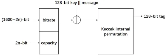
The construction of Keccak-MAC-nis illustrated in Figure 1. For the sake of convenience, we denote the state A after θ, ρ, and π in roundi (i ≥ 0) by Ai
θ, Aiρ andAiπ respectively. The input state of round i is denoted byAi. The
128-bit key is denoted byk, where ki represents theithbit ofk.
Fig. 1. Construction of Keccak-MAC-n
Observation 1 Since
A0θ[3][i] =A0[3][i]⊕( 4 M
y=0
A0[2][y])⊕( 4 M
y=0
(A0[4][y]≪1))
for 0 ≤i≤4,A0
θ[3][i] is independent of the 128-bit key. In other words, if we add bit conditions on A0
θ[3][i] , all of them are key-independent.
Then, we consider the influence of π◦ρ operation as shown in Figure 2. Consequently, Observation 2 can be obtained.
Fig. 2.π◦ρoperation
Observation 2 After π◦ρoperation, A0θ[2][i]andA0θ[4][t]are next to A0θ[3][j]
in each row, where(i, j, t)∈ {(2,3,4),(4,0,1),(1,2,3),(3,4,0),(0,1,2)}.
Our approach to determine the candidates for ordinary cube variables is heavily based on the two observations.
2.2 Cube Tester
Cube tester was first proposed by Aumasson et al. at FSE 2009 [1] after Dinur et al. introduced cube attack at Eurocrypt 2009 [6]. Different from standard cube attack, which aims at key extraction, cube tester performs non-randomness detection. In our paper, we only concentrate on a specific non-random behaviour, i.e. the cube sums are zero. To describe cube tester, we first recall the concept of cube attack as follows.
Theorem 2. [6]Given a polynomial f :{0,1}n→ {0,1}of degree d. Suppose
0< k < dand t denotes the monomialx0...xk−1. Then, f can be written as
f =t·Pt(xk, . . . , xn−1) +Qt(X),
where none of the terms of Qt(X) is divisible by t. Then the sum of f over all values of the cube (defined by t) is
X
x0∈C
t
f = X
x0∈C
t
If there exists such a cubeCtthat the following equation always hold, then
Ctcan be viewed as one type of cube tester [1], i.e. the sum over it always equals
zero.
X
x0∈C
t
f = X
x0∈C
t
f(x0, xk, . . . , xn−1) =Pt(xk, . . . , xn−1) = 0.
For example, consider the following polynomialf:
f(x0, x1, x2, x3) =x0x1+x1x2+x2x4+x1x3+x1x2x4.
Then, the following equation always hold:
X
(x0,x3)∈{0,1}2
f(x0, x1, x2, x3) = 0.
The reason is that that none of the monomial inf(x0, x1, x2, x3) is divisible by x0x3. However, if we sumf over all values of (x1, x2), then we can obtain the following equation:
X
(x1,x2)∈{0,1}2
f(x0, x1, x2, x3) = 1 +x4.
That is, the sum is dependent on the value ofx4.
2.3 Conditional Cube Tester
The concept of conditional cube tester was firstly proposed by Huang et al. [8] at Eurocrypt 2017. Their goal is to construct a key-dependent distinguisher. Therefore, they have to overcome the obstacle of how to involve the key information into the distinguisher. Motivated by this, they firstly classify the cube variables into two types: conditional cube variable and ordinary cube variable. The classification is based on the multiplying relations of the cube variables in the first two rounds as follows.
• Conditional cube variables can not multiply with each other after thesecond
round.
• Ordinary cube variables can not multiply with each other after thefirstround.
• Ordinary cube variables can not multiply with conditional cube variables after thesecond round.
Then, they develop a theorem to confirm the number of each type of the cube variables in order to establish a conditional cube tester, as specified below, whose proof is based on the relations of the cube variables in the first two rounds as above.
cube variables vp,vp+1, ..., vp+q−1, then the term v0v1...vp+q−1 will not appear
in the output polynomials of (n+ 2)-round Keccak sponge function.
To make conditional cube tester work, it is essential to introduce some conditions which will influence the above multiplying relations between the conditional cube variable and ordinary cube variable in the first two round. Specifically, only when all the introduced conditions hold will their multiplying relations be satisfied, thus making Theorem 1 work. Among the introduced conditions, the key-independent conditions can always be satisfied by controlling the input. For the key-dependent conditions, whether they are satisfied is detected by the conditional cube tester based on Theorem 1. To be more specific, the attack procedure can be briefly divided into three steps.
Step 1: Except for the cube variables in the input state, the attacker assigns a random value to the remaining part of it, while keeping the key-independent bit conditions satisfied.
Step 2: The attacker starts to exhaust all possible values of the cube variables and calculates the sum of all outputs.
Step 3: If the sum is zero, then the attacker knows that the key-dependent bit conditions are satisfied with an overwhelming probability and therefore he can extract some equations for the involved key bits. Otherwise, the attacker knows the key-dependent bit conditions do not hold. For this case, the attacker will flip some bits involved in the key-dependent bit conditions and located in the controllable part of the input state. Then, he goto Step 2 again.
The above procedure is only used to extract a small number of equations for the key bits. To recover the full key, the attacker will repeat the above procedure by changing the parameters of the conditions cube tester to extract more equations for the key bits. Finally, the attacker can solve the obtained equation system to recover some key bits. The remaining key bits can be recovered by brute force.
3
Tracing Algorithm
Several algorithms to determine the relations of cube variables in the first two rounds have been presented in [8]. In this section, we introduce a new method to achieve the same goal. We do not claim that our new method have any advantages over [8]. The purpose to use this new method is only to suit our programming. Before introducing how to determine the candidates for ordinary cube variables, we firstly describe how to trace the propagation of a variable inA0
θto A
1
π.
suppose M[i][J] = 1 (J ∈ {j0, . . . , j10}), then we construct a smaller matrix SM where SM[i][t] = jt for 0 ≤ t ≤ 10. Moreover, since the operation π◦ρ
is equivalent to a permutation of bit positions, an equivalent permutationP of size 1600 can be derived to express it.
To make the tracing algorithm more explicit, we should consider the internal state as a boolean vector denoted byV rather than a three-dimensional array. In addition, assume the internal state is an 1600-bit variable. For other sizes of the internal state, the procedure to trace the propagation is similar. For the sake of convenience, we denote the stateV afterθ,ρ, andπin roundi(i≥0) byVθi, Vρi andVπi respectively. The input state of roundiis denoted byVi.
Now we describe how to trace the propagation of the variable inA0θto A1π.
step 1. SupposeA0θ[x][y][z] contains a variable, we recordt0= (5x+y)×64 +z. step 2. Calculate how the variable inVθ0[t0] propagates throughπ◦ρoperation
withP. Consequently, we recordt1=P[t0].
step 3. According to the definition ofχ, afterι◦χ operation, three bits of V1 will contain the variable fromV0
π[t1]. We denote the corresponding three bit positions byt2,t3 andt4. Among the three bits, one bit will always contain this variable. The other two bits contain this variable depending on bit conditions. We classify these three bits into three types. The first type is the bit that always contains the variable. The second type is the bit that contains the variable depending on a key-independent bit condition. The third type is the bit that contains the variable depending on a key-dependent bit condition. Then, for each of the three bits, we trace how the variable in V1[pos] (pos ∈ {t2, t3, t4}) propagates to Vπ1
with Algorithm 1. The bit positions ofVπ1 containing the variable from
V1[pos] are stored in the the arrayf inalP osition.
Algorithm 1Tracing the influenced bit positions afterπ◦ρ◦θoperation 1: forrow in(0. . .1599)do
2: forcol in(0. . .10)do
3: if SM[row][col] =posthen 4: f inalP osition.push back(row)
5: break
Up until now, the propagation of the variable inA0θtoA1π is known, i.e. the
bit positions ofA1
π containing the variable fromA0θ are known and are classified
into three types. At last, we only need focus on how the cube variable in A0 propagates toA0
θ, which can be easily finished by considering the influence ofθ
operation.
Once knowing and recording how a variable propagates in the first two rounds with or without bit conditions to slow down this propagation, it is quite easy to determine their multiplying relations in the first two rounds. For example, suppose we know that A0
contains a different variable v00, then v00 will multiply with v0 after the first round. In the same way, suppose we know thatA1
π[x][y][z] contains a variablev0
and A1
π[x−1][y][z] contains a different variablev00, thenv00 will multiply with
v0 after the second round.
4
Finding Ordinary Cube Variables for Keccak-MAC-384
In this section, we will expand on the procedure to find sufficient ordinary cube variables for Keccak-MAC-384. First, the potential candidates for ordinary cube variables will be determined by carefully adding key-independent bit conditions to slow down its propagation. Then, we consider the multiplying relations of these candidates after the first round and deduce some contradictions. As will be shown, from these contradictions, we can efficiently determine how many ordinary cube variables can eventually survive.
4.1 Determining Candidates for Keccak-MAC-384
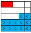
The initial state of Keccak-MAC-384 is shown in Figure 3 with 12 lanes set to 0. In the same way as [8,9,12], A[2][0][0] = A[2][1][0] = v0 is chosen as the conditional cube variable with four bit conditions (A0
θ[1][4][60] = 1,A0θ[1][0][5] =
1, A0
θ[3][1][7] = 0, A0θ[3][2][45] = 0) to slow down its propagation. Then, the
ordinary cube variables are set in the CP kernel. The complete procedure is as follows.
Fig. 3.Initial state of Keccak-MAC-384
• For the first column, we exhaust all 64 possible variablesA[0][1][i] =A[0][2][i] (0≤i≤63). Based onObservation 1 and 2, if we add bit conditions to slow down the propagation of the variables in this case, all of them are key-dependent bit conditions. Therefore, we do not add bit conditions. For each of these 64 possible variables, the tracing algorithm is applied to determine its multiplying relation with the chosen conditional cube variable in the first two rounds. Only those are selected as candidates that they do not multiply withv0 in the first two rounds.
• For the third column, we exhaust 63×3 possible variables A[2][0][i] = A[2][1][i], A[2][0][i] = A[2][2][i] and A[2][1][i] = A[2][2][i] (1 ≤ i ≤ 63). Based onObservation 1and2, we can add key-independent bit conditions on A0
θ[3][t] (0 ≤ t ≤ 4) to slow down the propagation of the variables.
To remove the redundant conditions, we add a condition only when it is necessary. In other words, if such a condition is not added and the variable satisfies the required relation withv0 in the first two rounds, this condition is not necessary and redundant. Moreover, if such a condition is added, the variable still does not satisfy the requirement, we filter this variable.
• For the forth column, we exhaust all 64 possible variables A[3][0][i] = A[3][1][i] (0 ≤ i ≤ 63) and process in the same way as the first column since there are no key-independent bit conditions to slow the propagation of variables.
• For the fifth column, we exhaust 64 possible variablesA[4][0][i] =A[4][1][i] (0≤i≤63). Based onObservation 1and2, we can add key-independent bit conditions to slow down the propagation of variables as the third column.
The candidates found with our method are presented in Table 2.
4.2 Discussion
Adding some bit conditions onA0θ[3][t] (0≤t≤4) as described above will cause the following bad cases.
Case 1: Contradiction of conditions will occur. Specifically, for the third column, the bit condition on a certain bit i of A0
θ[3][t0] is A0θ[3][t0][i] = 0. However, for the fifth column, the bit condition on a certain bit j of A0θ[3][t1] is A0θ[3][t1][j] = 1. If i = j and t0 = t1, the contradiction of conditions is detected. In other words, we can not choose both of their corresponding variables as the final ordinary cube variables. Moreover, ifA0θ[3][y0][z0] andA0θ[3][y1][z0] are added on different bit conditions for y0 >1, y1 >1, this is also a contradiction since A[3][y][z0] is set to a constant 0 for Keccak-MAC-384 fory >1.
Case 2: Contradiction between conditions and ordinary cube variables will occur. Specifically, for the forth column, some of A[3][0][i] = A[3][1][i] (0 ≤ i ≤ 63) will be chosen as candidates. The bad case is that A[3][0][t] =A[3][1][t] is chosen as a candidate andA0
θ[3][0][t] orA0θ[3][1][t]
is added on a condition.
Indeed, the second case can be processed in a simple way. After the candidates are determined, if a contradiction in the second case is detected, it implies that two ordinary variables multiplies with each other in the first round. For example, supposingA0
θ[3][0][t] is added on a condition andA[3][0][t] =A[3][1][t] is chosen
Table 2. Candidates for Keccak-MAC-384, where c is an adjustable constant over GF(2) for each variable.
A[0][1][i] =A[0][2][i] +c i 15 22 28 34 37 46 47 58 59 Variablev1 v2 v3 v4 v5 v6v7v8v9 A[1][1][i] =A[1][2][i] +c
i 7 15 20 26 30 38 39 40 52 54 57 Variablev10v11v12v13v14v15v16v17v18v19v20
A[2][0][i] =A[2][1][i] +c
i 1 8 12 14 15 20 23 25 28 41 42 43 45 50 52 53 61 62 63 Variable v21v22v23v24v25v26v27v28v29v30v31v32v33v34v35v36v37v38v39
Condition i=1:A0
θ[3][2][46] = 0 i=14:A0
θ[3][1][21] = 0
i=15:A0
θ[3][1][22] = 0 i=23:A
0
θ[3][2][4] = 0
i=25:A0
θ[3][1][32] = 0 i=42:A
0
θ[3][1][49] = 0
i=50:A0
θ[3][2][31] = 0 i=52:A
0
θ[3][1][59] = 0
i=63:A0
θ[3][1][6] = 0,A0
θ[3][2][44] = 0
A[3][0][i] =A[3][1][i] +c
i 3 4 9 13 15 23 30 35 39 40 46 56 57 Variablev40v41v42v43v44v45v46v47v48v49v50v51v52
A[4][0][i] =A[4][1][i] +c
i 3 5 8 10 12 14 20 22 25 30 31 35 38 41 47 57 58 62 63 Variable v53v54v55v56v57v58v59v60v61v62v63v64v65v66v67v68v69v70 v71
Condition i=3:A0
θ[3][0][59] = 1 i=8:A0
θ[3][0][0] = 1
i=20:A0
θ[3][0][12] = 1 i=22:A0
θ[3][0][14] = 1
i=25:A0
θ[3][0][17] = 1 i=30:A0
θ[3][4][1] = 1, A0
θ[3][0][22] = 1
i=35:A0
θ[3][4][6] = 1, A0
θ[3][0][27] = 1 i=38:A0
θ[3][4][9] = 1
i=41:A0θ[3][0][33] = 1 i=57:A0θ[3][0][49] = 1
A[2][0][i] =A[2][2][i] +c
i 1 5 6 14 15 16 20 21 27 30 33 38 39 40 41 46 51 52 57 61 62 Variable v72v73v74v75v76v77v78v79v80v81v82v83v84v85v86v87v88v89v90v91v92
Condition i=1:A0
θ[3][3][23] = 0 i=14:A0
θ[3][1][21] = 0, A0
θ[3][3][36] = 0
i=15:A0
θ[3][1][22] = 0 i=20:A0
θ[3][3][42] = 0
i=30:A0
θ[3][1][37] = 0 i=33:A0
θ[3][3][55] = 0
i=38:A0
θ[3][1][45] = 0 i=40:A0
θ[3][1][47] = 0
i=46:A0
θ[3][1][53] = 0 i=52:A0
θ[3][1][59] = 0
i=57:A0
θ[3][1][0] = 0 i=62:A0
θ[3][3][20] = 0
A[2][1][i] =A[2][2][i] +c
i 1 11 14 15 18 19 20 24 41 52 56 58 61 62 Variable v93v94v95v96v97v98v99v100 v101 v102v103v104v105v106
Conditioni=1:A0
θ[3][2][46] = 0, A0
θ[3][3][23] = 0 i=14:A0
θ[3][3][36] = 0
i=18:A0
θ[3][2][63] = 0 i=20:A
0
θ[3][3][42] = 0
i=56:A0θ[3][3][14] = 0 i=62:A
0
each other in the first round. Benefiting from this new property, we do not have to process the second bad case and only need concentrate on the relation of the candidates in the first round as well as the contradiction caused by conditions.
4.3 Deducing Contradictions
The contradictions of candidates are deduced from two cases. The first case is that variables multiply with each other in the first round. The second case is that there is contradiction of conditions. The contradictions deduced are displayed in Table 3. In this table,vi{vj0, ..., vjn} meansvi can not be chosen with any of
{vj0, ..., vjn} as the final candidates at the same time. We count the times that each variable appears in these contradictions and do not choose the one which appears more than one time as marked in red and blue. However, although some variables appear two times as marked in green in this table, we can still choose them. Therefore, for the obtained contradictions, at most 28 variables can be derived. Moreover, there are 56 fully free variables, i.e. there are no contradictions on them.
Table 3. Contradictions of candidates
v1{v70} v2{v54,v63} v3{v19} v5{v59} v7{v62}
v8{v12, v53, v66}v11{v77} v12{v79} v13{v80} v15{v84}
v16{v85} v17{v86, v101}v20{v104}v22{v44} v27{v46}
v29{v47} v34{v52} v37{v41} v41{v57, v91}v43{v74}
v45{v63,v77} v46{v65} v48{v67} v49{v82} v50{v84}
Observe that we consider the third column under three cases, which will cause two problems. Specifically, ifA[2][0][t] =A[2][1][t] +c,A[2][0][t] =A[2][2][t] +c andA[2][1][t] =A[2][2][t]+care chosen simultaneously, only two variables rather than three variables can be obtained. In this case, we should change the variables as A[2][0][t] =vx0, A[2][1][t] =vx1, A[2][2][t] =vx0+vx1+c. This is due to that
the ordinary cube variables are set in the CP kernel. According to Table 2, there are 8 possible values for t and they are{1,14,15,20,41,52,61,62}. Therefore, for the worst case, we can finally obtain 28 + 56−8 = 76 ordinary cube variables, which is much larger than the required number (63) to mount key-recovery attack on 7-round Keccak-MAC-384.
On the other hand, if two ofA[2][0][t] =A[2][1][t] +c,A[2][0][t] =A[2][2][t] + c, A[2][1][t] = A[2][2][t] +c are chosen simultaneously, we should change the variables asA[2][0][t] =vx0, A[2][1][t] =vx1, A[2][2][t] =vx0+vx1+c.
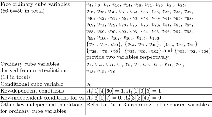
Table 4.One choice of ordinary cube variables for Keccak-MAC-384
Free ordinary cube variables v4,v6,v9,v10,v14,v18,v21,v23,v24,v25, (56-6=50 in total) v26,v28,v30,v31,v32,v33,v35,v36,v38,v39,
v40,v42,v51,v55,v56,v58,v60,v61,v64,v68,
v69,v71,v72,v73,v75,v76,v78,v81,v83,v87,
v88,v89,v90,v92,v93,v94,v95,v96,v97,v98,
v99,v100,v102,v103,v105,v106.
{v21,v72,v93},{v24,v75,v95},{v25,v76,v96} {v26,v78,v99},{v35,v89,v102}and{v38,v92,v106} provide two variables respectively.
Ordinary cube variables v1,v54,v63,v3,v5,v7,v53,v66,v11,v79, derived from contradictions v13,v15,v16
(13 in total)
Conditional cube variable v0
Key-dependent conditions A0θ[1][4][60] = 1, A
0
θ[1][0][5] = 1.
Key-independent conditions forv0 A0θ[3][1][7] = 0, A
0
θ[3][2][45] = 0.
Other key-independent conditions Refer to Table 3 according to the chosen variables. for ordinary cube variables
5
Finding Ordinary Cube Variables for Keccak-MAC-512
Although 32-dimensional cube variables have been found with MILP to establish the 6-round conditional cube tester for Keccak-MAC-512 and the time complex-ity is practical, we want to explain how to apply our method to achieve the same goal. This is for a better understanding of the differences between our method and others based on MILP. Now, we expand on how to find sufficient cube variables for Keccak-MAC-512.
In a similar way for Keccak-MAC-384, 32 candidates for ordinary cube vari-ables are discovered as displayed in Table 5. The corresponding contradictions are as follows.
v2{v24}, v7{v26}, v9{v27}, v14{v32}, v17{v21}.
Therefore, there will be 32−5 = 27 possible ordinary cube variables in total if the ordinary cube variables are set only in the CP kernel. As a result, we can not mount key-recovery attack on 6-round Keccak-MAC-512, which requires 31 ordinary cube variables if onlyv0 is chosen to be the conditional cube variable. Based on [12], the variables which multiply withv0only in the second round can be leveraged as well. For an intuitive example, suppose one variable vx0
multiplies with v0 only in the second round and the multiplying bit position is p0. If another variable vx1 multiplies withv0 only in the second round and the multiplying bit position isp0as well, then settingvx0 =vx1will cause the already
filtered two variables become one possible variable. Then, the goal becomes how to find these possible variables.
SupposeA0
θ[i][j][k] contains a variable, then afterχoperation, three bits will
Table 5. Candidates for Keccak-MAC-512, where c is an adjustable constant over GF(2) for each variable.
A[2][0][i] =A[2][1][i] +c
i 1 8 12 14 15 20 23 25 28 41 42 43 45 50 52 53 61 62 63 Variable v1v2v3v4v5v6 v7 v8 v9v10v11v12v13v14v15v16v17v18 v19
Condition i=1:A0
θ[3][2][46] = 0 i=14:A0
θ[3][1][21] = 0
i=15:A0
θ[3][1][22] = 0 i=23:A0
θ[3][2][4] = 0
i=25:A0
θ[3][1][32] = 0 i=42:A0
θ[3][1][49] = 0
i=50:A0
θ[3][2][31] = 0 i=52:A0
θ[3][1][59] = 0
i=63:A0
θ[3][1][6] = 0, A0
θ[3][2][44] = 0
A[3][0][i] =A[3]1][i] +c
i 3 4 9 13 15 23 30 35 39 40 46 56 57 Variablev20v21v22v23v24v25v26v27v28v29v30v31v32
bits, one bit will always contain this variable and the other two bits contain this variable depending on the conditions. We classify the three bits into three types.
Type-1: It always contains this variable.
Type-2: It contains this variable depending on a key-independent bit condition.
Type-3: It contains this variable depending on a key-dependent bit condition.
Then, we trace how the three bits propagate to the second round with the tracing algorithm. Specifically, we trace theType-1bit and record the influenced bits of A1π multiplying withv0in the second round. For the Type-2andType-3bits, we process in the same way. The recorded bits forType-1,Type-2andType-3
are defined as core bits, independent-key bits and key-dependent bits. Since our focus is the minimal key-dependent conditions, once the key-dependent bits are detected, the corresponding variable should not be chosen as a candidate.
With the above method, we reconsider the filtered ordinary cube variables set in the CP kernel. Besides, the variables set to a single bit are also considered. The final result obtained is displayed in Table 6.
For a better understanding of this table, we take the variable A[3][1][8] as instance. For the first column, it means A[3][1][8] is set to be a variable. For the second column, it means 5 bits of A1
π will multiply with v0 only in the second round. For the third column,{656,1003} means the two bits of A1
π, i.e.
A1
π[0][2][16] and A1π[0][3][43], will multiply with v0 only in the second round depending on the same key-independent bit condition. The last column means A[3][1][8] can not be chosen as a variable with any of v1 and v31 in Table 5 simultaneously.
According to Table 6, at most three more possible ordinary cube variables can be obtained. One choice is as follows:
A[3][0][58] =A[3][1][58] =A[2][0][24] =A[2][1][24] =ve0,
A[3][0][61] =ve1, A[3][1][61] =ve2,
A[2][0][26] =A[2][1][26] =ve3, ve3 =ve2+ve1
A[2][0][46] =A[2][1][46] =ve2.
According to Table 6, adding A[2][0][37] = A[2][1][37] = ve2 to the above
variables and converting the bit conditionA0
θ[3][1][53] = 0 intoA
0
θ[3][1][53] = 1 is
also possible. However, it can not help improve the number of possible variables. In fact, there are many interesting cases. For example, ifA[3][0][60] =A[3][1][60] does not multiply withv16in the first round, we can obtain one more candidate. For the third row, if {652,1109} does not depend on the same condition, then we can add one key-independent bit condition to prevent the propagation to the 652-nd bit and another key-independent bit condition to allow the propagation to the 1109-th bit ofA1π.
Table 6.Possible candidates for Keccak-MAC-512
Possible Variables Core Bits Key-independent Contradictions Bits
A[2][0][4] =A[2][1][4] 1540
A[2][0][5] =A[2][1][5] 1109 {652,1109}
A[2][0][9] =A[2][1][9] 848,467 {656,1003}
A[2][0][13] =A[2][1][13] 652,1109
A[2][0][16] =A[2][1][16] 1472 515 v25
A[2][0][24] =A[2][1][24] 515
A[2][0][26] =A[2][1][26] 665
A[2][0][29] =A[2][1][29] 71,1032 241
A[2][0][33] =A[2][1][33] 491 v29
A[2][0][35] =A[2][1][35] 1131,42 1242
A[2][0][37] =A[2][1][37] 1040
A[2][0][46] =A[2][1][46] 903 1040
A[2][0][51] =A[2][1][51] 767,1160
A[2][0][54] =A[2][1][54] 1510
A[2][0][57] =A[2][1][57] 170 205
A[2][0][60] =A[2][1][60] 1280 1540 v20
A[3][0][41] =A[3][1][41] 113
A[3][0][43] =A[3][1][43] 848
A[3][0][50] =A[3][1][50] 42 v12
A[3][0][58] =A[3][1][58] 515
A[3][0][60] =A[3][1][60] 665 v16
A[3][0][61] =A[3][1][61] 903
A[3][1][8] 170,848,467,1382,1003{656,1003},{903},{1237} v1, v31
A[3][0][32] 491,903,1382 {13},{848},{775} v29
A[3][0][61] 665 {42},{1348}
A[3][1][61] 903,665 {42},{1348}
Then we test whethervei (0≤i≤3) multiplies with each other in the first round and check whether the three bit conditions to slow down the propagation ofve1 andve2 are contradict with the conditions in Table 5. It is shown that the
way why [12] can only discover the same number of such ordinary variables with a solver. However, to mount key-recovery attack on 6-round Keccak-MAC-512, we need 31 ordinary cube variables. Thus, we try to search ordinary cube variables set in the CP kernel with only one key-dependent bit condition, which satisfy the required relation with v0 and the chosen 32 + 4 = 36 candidates for ordinary cube variables. Our searching result is displayed in Table 7. Thus, there are many possible choices for 31 ordinary cube variables, i.e. at least 25× 12. The verification can be found athttps://github.com/Crypt-CNS/Keccak_ ConditionalCubeAttack.git.
Table 7.Candidates for Keccak-MAC-512 with one key-dependent bit condition
Variable Conditions
A[2][0][11] =A[2][1][11]A0
θ[1][4][7] = 1
A[2][0][19] =A[2][1][19]A0
θ[1][4][15] = 1
A[2][0][21] =A[2][1][21]A0
θ[1][0][26] = 1,A0θ[3][2][2] = 0
A[2][0][22] =A[2][1][22]A0
θ[1][0][27] = 1
A[2][0][30] =A[2][1][30]A0
θ[3][1][37] = 0,A0θ[1][0][35] = 1
A[2][0][34] =A[2][1][34]A0
θ[1][0][39] = 1,A0θ[3][2][15] = 0
A[2][0][44] =A[2][1][44]A0θ[3][1][51] = 0,A0θ[1][0][49] = 1
A[2][0][56] =A[2][1][56]A0θ[1][4][52] = 1,A0θ[3][1][63] = 0
A[3][0][12] =A[3][1][12]A0θ[4][1][20] = 0
A[3][0][20] =A[3][1][20]A0θ[4][2][36] = 0
A[3][0][29] =A[3][1][29]A0θ[2][4][60] = 1
A[3][0][34] =A[3][1][34]A0θ[2][4][1] = 1
6
Recovering Full Key
In this section, a new slightly improved way to recover 128-bit key for Keccak-MAC is presented by removing unnecessary iterations of conditional cube tester. In [8], 64 iterations of the conditional cube tester were used to recover the 128-bit key for Keccak-MAC-256. For each iteration, it costs 264+2= 266to recover 2-bit key. Observe that once there are only a few key bits to be recovered, there is no need to iterate the conditional cube tester since each iteration is costly and only 2 bits are recovered.
Taking Keccak-MAC-128/256 for instance, for the 64-dimensional cube variable [8], after 31 iterations in z-axis of the conditional cube tester, 62 bits of key can be recovered. Then, the remaining 66 bits can be recovered by brute force. Therefore, the time complexity is improved to 266×31 + 266 = 271 from 272. Similarly, for the 64-dimensional cube variables in Table 4, we can recover the 128-bit key for 7-round Keccak-MAC-384 with time complexity 271.
For the conditional cube attack on 6-round Keccak-MAC-512, we choose A[2][0][11] = A[2][1][11] in Table 7 as the ordinary cube variable with one key-dependent bit condition A0
in [12]. For our choice, only 31 iterations in z-axis is enough. Then, 3×31 = 93 bits can be recovered with time complexity 232+3×31 = 235×31. The remaining 128−93 = 35 bits can be recovered by brute force. The order to recover 93 bits of key with conditional cube tester is shown in Table 8. Therefore, the total time complexity becomes 235×31 + 235 = 240. However, the time complexity is estimated as d128
3 e ×2
25+3 = d128 3 e ×2
35 = 240.4 in [12], which implies 64 iterations of the conditional cube tester are used to recover the 128-bit key.
Table 8.The order to recover 93 bits of key with conditional cube tester
(k0, k53, k62⊕k126), (k1, k54, k63⊕k127), (k2, k55, k0⊕k64), (k3, k56, k1⊕k65), (k4, k57, k2⊕k66), (k5, k58, k3⊕k67), (k6, k59, k4⊕k68), (k7, k60, k5⊕k69), (k8, k61, k6⊕k70), (k9, k62, k7⊕k71), (k10, k63, k8⊕k72), (k22, k11, k20⊕k84), (k23, k12, k21⊕k85), (k24, k13, k22⊕k86), (k25, k14, k23⊕k87), (k26, k15, k24⊕k88), (k27, k16, k25⊕k89), (k28, k17, k26⊕k90), (k29, k18, k27⊕k91), (k30, k19, k28⊕k92), (k31, k20, k29⊕k93), (k32, k21, k30⊕k94), (k44, k33, k42⊕k106), (k45, k34, k43⊕k107), (k46, k35, k44⊕k108), (k47, k36, k45⊕k109), (k48, k37, k46⊕k110), (k49, k38, k47⊕k111), (k50, k39, k48⊕k112), (k51, k40, k49⊕k113), (k52, k41, k50⊕k114).
7
Comparison with Previous Work
Our work is heavily based on [8]. However, Huang et al. did not consider the potentially useful key-independent bit conditions to slow down the propagation of ordinary cube variables [8].
As for [9], it seems that the key-independent bit conditions have been considered. However, it is strange that Li et al. found 63 ordinary cube variables with 6 key-dependent bit conditions for Keccak-MAC-384, while we can find much more ordinary cube variables without key-dependent bit conditions, i.e. at least 76 variables. Besides, Li et al. only found 25 ordinary cube variables set in the CP kernel for Keccak-MAC-512, while we can find 32−5 = 27 ordinary cube variables set in the CP kernel. Therefore, we guess that the key-independent bit conditions were not fully leveraged in [9].
affect the time complexity to recover the key. However, from the scientific point, if there is a more accurate answer, why not choose it?
In addition, a new slightly improved approach to recover the 128-bit key is introduced. This is based on the observation that many iterations of the conditional cube tester are costly once a few bits of key are left. Consequently, we improve the conditional cube attack on 7-round Keccak-MAC-128/256/384 and 6-round Keccak-MAC-512.
8
Conclusion
An algorithm to search ordinary cube variables for Keccak-MAC is developed. The first step is to identify a small region of potential candidates by making full use of the key-independent bit conditions. Then, these candidates are further filtered according to their relations after the first round with an efficient approach. In this way, sufficient ordinary cube variables can be discovered to establish the conditional cube tester. Combined with the new slightly improved way to recover the key, the time complexity of the conditional cube attack on 7-round Keccak-MAC-128/256/384 and 6-round Keccak-MAC-512 are improved to 271 and 240 respectively.
Acknowledgement We thank the anonymous reviewers of IWSEC 2019 for their insightful comments and suggestions. Fukang Liu and Zhenfu Cao are sup-ported by National Natural Science Foundation of China (Grant No.61632012, 61672239). Gaoli Wang is supported by the National Natural Science Foundation of China (No. 61572125) and National Cryptography Development Fund (No. MMJJ20180201).
References
1. Jean-Philippe Aumasson, Itai Dinur, Willi Meier, and Adi Shamir. Cube testers and key recovery attacks on reduced-round MD6 and Trivium. In Fast Software Encryption, 16th International Workshop, FSE 2009, Leuven, Belgium, February 22-25, 2009, Revised Selected Papers, pages 1–22, 2009.
2. Guido Bertoni, Joan Daemen, Micha¨el Peeters, and Gilles Van Assche. The Keccak reference, 2011. http://keccak.noekeon.org.
3. Wenquan Bi, Xiaoyang Dong, Zheng Li, Rui Zong, and Xiaoyun Wang. MILP-aided cube-attack-like cryptanalysis on Keccak keyed modes. Cryptology ePrint Archive, Report 2018/075, 2018. https://eprint.iacr.org/2018/075.
4. Itai Dinur, Orr Dunkelman, and Adi Shamir. New attacks on Keccak-224 and Keccak-256. In Fast Software Encryption - 19th International Workshop, FSE 2012, Washington, DC, USA, March 19-21, 2012. Revised Selected Papers, pages 442–461, 2012.
Annual International Conference on the Theory and Applications of Cryptographic Techniques, Sofia, Bulgaria, April 26-30, 2015, Proceedings, Part I, pages 733–761, 2015.
6. Itai Dinur and Adi Shamir. Cube attacks on tweakable black box polynomials. In Advances in Cryptology - EUROCRYPT 2009, 28th Annual International Conference on the Theory and Applications of Cryptographic Techniques, Cologne, Germany, April 26-30, 2009. Proceedings, pages 278–299, 2009.
7. Jian Guo, Meicheng Liu, and Ling Song. Linear structures: Applications to cryptanalysis of round-reduced Keccak. InAdvances in Cryptology - ASIACRYPT 2016 - 22nd International Conference on the Theory and Application of Cryptology and Information Security, Hanoi, Vietnam, December 4-8, 2016, Proceedings, Part I, pages 249–274, 2016.
8. Senyang Huang, Xiaoyun Wang, Guangwu Xu, Meiqin Wang, and Jingyuan Zhao. Conditional cube attack on reduced-round Keccak sponge function. InAdvances in Cryptology - EUROCRYPT 2017 - 36th Annual International Conference on the Theory and Applications of Cryptographic Techniques, Paris, France, April 30 - May 4, 2017, Proceedings, Part II, pages 259–288, 2017.
9. Zheng Li, Wenquan Bi, Xiaoyang Dong, and Xiaoyun Wang. Improved conditional cube attacks on Keccak keyed modes with MILP method. In Advances in Cryptology - ASIACRYPT 2017 - 23rd International Conference on the Theory and Applications of Cryptology and Information Security, Hong Kong, China, December 3-7, 2017, Proceedings, Part I, pages 99–127, 2017.
10. Kexin Qiao, Ling Song, Meicheng Liu, and Jian Guo. New collision attacks on round-reduced Keccak. In Advances in Cryptology - EUROCRYPT 2017 - 36th Annual International Conference on the Theory and Applications of Cryptographic Techniques, Paris, France, April 30 - May 4, 2017, Proceedings, Part III, pages 216–243, 2017.
11. Ling Song and Jian Guo. Cube-attack-like cryptanalysis of round-reduced Keccak using MILP. IACR Trans. Symmetric Cryptol., 2018(3):182–214, 2018.
12. Ling Song, Jian Guo, Danping Shi, and San Ling. New MILP modeling: Improved conditional cube attacks on Keccak-based constructions. In Advances in Cryptology - ASIACRYPT 2018 - 24th International Conference on the Theory and Application of Cryptology and Information Security, Brisbane, QLD, Australia, December 2-6, 2018, Proceedings, Part II, pages 65–95, 2018.
13. Ling Song, Guohong Liao, and Jian Guo. Non-full sbox linearization: Applications to collision attacks on round-reduced Keccak. In Advances in Cryptology -CRYPTO 2017 - 37th Annual International Cryptology Conference, Santa Barbara, CA, USA, August 20-24, 2017, Proceedings, Part II, pages 428–451, 2017. 14. Xiaoyun Wang, Yiqun Lisa Yin, and Hongbo Yu. Finding collisions in the full
SHA-1. In Advances in Cryptology - CRYPTO 2005: 25th Annual International Cryptology Conference, Santa Barbara, California, USA, August 14-18, 2005, Proceedings, pages 17–36, 2005.