Bayesian Inference for High Dimensional Models: Convergence Properties and Computational Issues.

(1)

ABSTRACT

BANERJEE, SAYANTAN. Bayesian Inference for High Dimensional Models: Convergence Properties and Computational Issues. (Under the direction of Subhashis Ghoshal.)

This dissertation focuses on Bayesian inference for high-dimensional models, including

estimation of the mean in different regression models, and estimation of precision matrices for

high dimensional random variables. Along with studying theoretical properties of posterior

distributions, we also develop computational methods for efficient and fast model assessment.

In Chapter 2, we consider a fast Bayesian variable selection method for generalized

addi-tive partial linear models. The functions in the non-parametric addiaddi-tive part of the model are

expanded in a B-spline basis and multivariate Laplace prior put on the coefficients with point

mass at zero. The coefficients corresponding to the strictly linear components are assigned a

univariate Laplace prior with point mass at zero. The prior times the likelihood is

mathemati-cally intractable but we find an approximation by expansion around the posterior mode, which

is the group lasso solution in generalized linear model setting for the choice of prior. We thus

completely avoid Markov Chain Monte Carlo (MCMC) or any other time consuming sampling

based methods, hence leading to quick assessment of various posterior model probabilities.

This technique is applied to the high-dimensional situation where the number of parameters

may exceed the number of observations. We evaluate the performance of the Bayesian method

by conducting simulation studies and real data analyses.

In Chapter 3, we consider Bayesian estimation of a p×p precision matrix, when p can be much larger than the available sample size n. It is well known that consistent estimation in such ultra-high dimensional situations requires regularization such as banding, tapering or

thresholding. We consider a banding structure in the model and induce a prior distribution

(2)

only when two vertices are within a given distance. For a proper choice of the order of graph,

we obtain the convergence rate of the posterior distribution and Bayes estimators based on the

graphical model in theL∞-operator norm uniformly over a class of precision matrices, even if the true precision matrix may not have a banded structure. Along the way to the proof, we also

compute the convergence rate of the maximum likelihood estimator (MLE) under the same set

of conditions, which is of independent interest. The graphical model based MLE and Bayes

estimators are automatically positive definite, which is a desirable property not possessed by

some other estimators in the literature. We also conduct a simulation study to compare finite

sample performance of the Bayes estimators and the MLE based on the graphical model with

that obtained by using a Cholesky decomposition of the precision matrix. Finally, we discuss

a practical method of choosing the order of the graphical model using the marginal likelihood

function.

In Chapter 4, we consider a similar problem of estimating a sparse precision matrix of

a multivariate Gaussian distribution, including the case where the dimension p exceeds the sample sizen, but now without the assumption of a banding structure in the model. A popular non-Bayesian method of estimating a graphical structure is given by the graphical lasso. In this

chapter, we consider a Bayesian approach to the problem. We use priors which put a mixture

of a point mass at zero and certain absolutely continuous distribution on off-diagonal elements

of the precision matrix. Hence the resulting posterior distribution can be used for graphical

structure learning. The posterior convergence rate of the precision matrix is obtained. The

posterior distribution of different graphical models is extremely cumbersome to compute. We

propose a fast computational method for approximating the posterior probabilities of various

graphs using the Laplace approximation method by expanding the posterior density around the

posterior mode, which is the graphical lasso by our choice of the prior distribution. We also

(3)

(4)

Bayesian Inference for High Dimensional Models: Convergence Properties and Computational Issues

by

Sayantan Banerjee

A dissertation submitted to the Graduate Faculty of North Carolina State University

in partial fulfillment of the requirements for the Degree of

Doctor of Philosophy

Statistics

Raleigh, North Carolina

2014

APPROVED BY:

Peter Bloomfield Soumendra Nath Lahiri

Brian Reich Subhashis Ghoshal

(5)

DEDICATION

To Adrija,

to my parents,

and

(6)

BIOGRAPHY

Sayantan Banerjee was born to two wonderful parents, Chandan Kumar Banerjee and

Malo-bika Banerjee, in the city of Chandannagar, West Bengal, India. He started schooling in The

Study Home, before getting admitted to Sri Aurobindo Vidyamandir, one of the best schools in

the state. He spent the next ten years (1993-2003) of his academic life there, gradually

grow-ing to the man of today. After spendgrow-ing two years for higher secondary studies at Kanailal

Vidyamandir, he pursued his undergraduate studies in Statistics at St Xavier’s College, Kolkata

(2005-2008). Sayantan got admission at the prestigious Indian Statistical Institute, Kolkata for

his Master’s in Statistics (2008-2010). With a motto to build a career in research, he joined

the PhD program in the Department of Statistics at North Carolina State University in August

2010. Apart from research work, Sayantan takes interest in a variety of other activities, ranging

from literature to sports. He is an avid reader, writes occasionally, plays football (soccer, in

US) and cricket, and wanders off often with his camera in hand, for his love of photography

and travel. He loves to eat, is a tea-freak, and takes a passionate interest in railways. He met

his soulmate Adrija Chatterjee in 2011, who remain his best treasure since then. Sayantan

will be joining the University of Texas MD Anderson Cancer Center at Houston, Texas as a

(7)

ACKNOWLEDGEMENTS

I would like to thank my advisor, Professor Subhashis Ghoshal, for his immense help in the

entire journey of my research career here at NC State. Without his help, advice, and mentoring,

this wouldn’t have been possible. His patience and sincerity makes him one of the best advisors

one could ever have. The experience of working with him has been great, and I have learnt a

lot from the one-to-one conversations we have had over the past few years. He has been most

accommodating, caring, and had taken the relationship beyond the walls of academia, mixing

it with good humor. Our discussions went beyond the titbits of epsilons and deltas, bringing in

chats ranging from cricket to food and much more.

I would also like to thank all the other members in my thesis committee, namely, Professors

Peter Bloomfield, Soumendra Nath Lahiri and Brian Reich, for careful review and providing

valuable suggestions in improving the contents of this thesis. They have always been very

generous to provide their valuable time and energy in the entire process. Also I would like to

extend my sincere thanks to all the other Professors in the department for giving a platform of

high quality research and training environment through their professional activities. Not only

the Professors, I should thank all the staff, especially Alison McCoy and Adrian Blue, for their

excellent service to the department and for making our lives easier.

Life as a graduate student is always difficult. Mine was no exception. The first journey to

US itself had been a remarkable story for me. Nevertheless, the first few months would have

been much difficult if there weren’t the helping hands of Dr Sujit Ghosh and his wife Chumki

di. I would forever remain indebted to their help and care. Also I would like to thank Dr Arnab

Maity for all the valuable guidance he has provided from the very beginning.

My days here in the US would have been much dim but for the presence of two of the most

(8)

presence itself provided a sense of security. I have always felt blessed with their ever extending

hands of love and care. Thank you!

I remain indebted towards all the teachers I have come across in my entire academic life.

I extend my heartiest gratitude to these people who laid the foundations of success during my

school days. Specially I should mention the roles of Shanti Ranjan Pal and Srikumar Ghosh,

the two people who inspired me to choose a career in Statistics, remaining a guiding light

throughout; and two of my most favorite teachers, Patralekha Basu and Gunamay Burman, for

all I have learnt from them. I was also blessed with the best of the teachers during my college

days. I would specially like to thank Amit Ghosh and Surupa Chakraborty at St Xavier’s,

and Tapas Samanta, Sumitra Purkayastha, Smarajit Bose at ISI Kolkata, for providing utmost

help and guidance. And last but not the least, I would like to thank the great Partho Sarathi

Chakrabarti from RKM Narendrapur for showing the path of effectively teaching Statistics at

the undergraduate level. His style of teaching, ability to think about a statistical problem still

remain a benchmark for me to follow as a teacher in the future.

I have been blessed with friends in this great department, for whom the department

con-tinues to be a home away from home. My sincere gratitude to all of them, including Weining

Shen, Seung Jun Shin, Meng Li, Bo Zhang, Woo Sung Jang, Clemontina Davenport,

Kas-turi Talapatra, Cassie Kozyrkov – for all the good days. I take the opportunity to bid all of

them good-bye with a big thanks through here. I wish all of them a huge success in life. Not

only in my department, I also have been lucky enough to be amongst a handsome number

of friends in the locality from other departments and also from neighboring universities like

UNC Chapel Hill and Duke University, who continued to provide ample support throughout

the days here – Lopamudra Kundu, for her deep caring love as a sister; Anjishnu Banerjee, for

the brain-storming Bayesian sessions and cricket; Shuva Gupta, for all the help and concerns;

(9)

Pal Majumdar, Sujatro Chakladar, Priyam Das, Pradip Tarafdar, Chiranjit Mukherjee, for

ex-tending their hands of friendship always – in normal times, and in times of crisis. And I should

not forget to mention the role of Ayan Das Gupta, who treated me more than a brother and

provided constant support (along with his culinary skills) during the two years he spent here at

Raleigh.

School days have remained the best of the days from yesteryear. My childhood was

awe-some for my wonderful school Sri Aurobindo Vidyamandir, where I have spent the most vital

10 years of my life as a student. I will be ever grateful for all the love, support, care and

fun my school had provided me. It would be a great mistake if I do not acknowledge the

role of my friends in this regard, for accompanying me growing to the adult of today. I owe

a lot to all my school friends; especially I would like to mention Nayan Banerjee, Arghadip

Samaddar, Debanjan Mitra, Dipanjan Das, Arpan Sinha, Anindya Ganguly, Soham Mukherjee,

Avinandan Sthanpati, Soumyadip Neogy, Sourav Ghosh and Soham Das, for all their love and

support. I would also like to thank my friends from my college days. The five years I have

spent at St Xavier’s and ISI would have been incomplete without them – Abirbhab

Bandyopad-hyay, for being more than a best friend, and without the continued mental support of whom I

wouldn’t have sustained the journey this far; Soumya Banerjee, Shankhadeep Senchowdhury,

Subhajyoti Sen, for always being the fun guys around; Sarani Sengupta, for all the care and

support; Parichoy Pal Chowdhury, aka PPC, for just being himself; Sandipan Roy, Soumalya

Mukhopadhyay, Projjwal Das, Sohini Dasgupta, for defining an epitome of eternal friendship.

And I would also like to thank two of my junior friends, Debankur Mukherjee and Abhijoy

Saha, for standing by my side always. I have learnt a lot from you two.

There are no shortcuts to success without working hard. I hereby express my heartiest

gratitude to two people who have always remained a role-model to me in this regard – Satyajit

(10)

role they have played in motivating at times when everything seemed to fall apart. I turned to

them in happiness, and in times of sorrow. And I would like to add a little vote of thanks for

the Indian Cricket team and Manchester United Football Club for all the happiness they have

provided since childhood.

This thesis wouldn’t have seen light if not for the wonderful family I have, who have

con-stantly motivated me throughout my life. Words fall short for the contribution of my father,

Chandan Kumar Banerjee, who laid the foundation of whatever interest I have in

mathemati-cal sciences. The same goes for my mother, Malobika Banerjee, who taught me to read and

write, and without whose love, care and blessings I couldn’t have come this far. Thanks

‘Meso-mashai’, Dr Chittaranjan Mukherjee, for truly respecting and supporting my decision to pursue

a research career in Statistics, instilling the confidence in me when some significant others

doubted. I would also thank all my uncles, aunts, cousins and grandparents for being

support-ive always. Their good wishes will remain the motivating forces for the days to come. A lot

of thanks goes to my mother-in-law, Santasri Chatterjee, for all her love and blessings; and my

father-in-law Tara Prasad Chatterjee, for all his best wishes. Amongst all the happiness, I spare

some moments for my maternal grandparents, Late Narayan Chandra Chattopadhyay and Late

Mira Chattopadhyay, and my very dear brother Late Arindam Mukherjee, who couldn’t live to

see this day. I miss you.

Finally, my heartiest thanks goes to the one without whom I am incomplete; my better half,

Adrija Chatterjee. She has been prolific in providing more than her soul to help me breeze

through the entire journey. She might have lived miles away most of the times, but never let

me feel alone even for a moment. Without her constant encouragement and love, the stressful

(11)

LIST OF TABLES

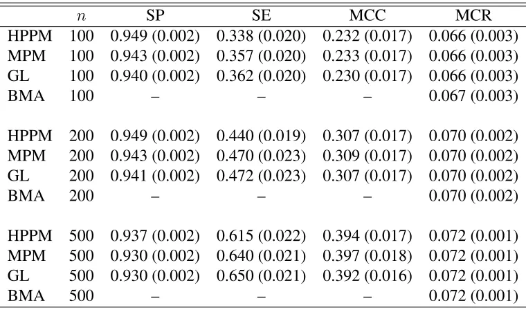
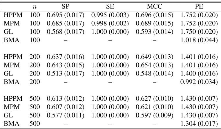
Table 2.1 Table corresponding to independent predictors,p= 10, s= 10in GAPLM (logistic regression). Figures in parentheses represent respective standard errors. . . 37 Table 2.2 Table corresponding to independent predictors,p= 10, s= 10in GAPLM

with misspecification. Figures in parentheses represent respective standard errors. . . 38 Table 2.3 Table corresponding to independent predictors,p= 100, s= 100in GAPLM

(logistic regression). Figures in parentheses represent respective standard errors. . . 39 Table 2.4 Table corresponding to independent predictors,p= 100, s= 100in GAPLM

with misspecification. Figures in parentheses represent respective standard errors. . . 40 Table 2.5 Table corresponding to independent predictors,p = 10, s = 10 in APLM.

Figures in parentheses represent respective standard errors. . . 41 Table 2.6 Table corresponding to independent predictors,p= 100, s= 100in APLM.

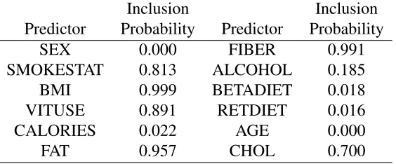
Figures in parentheses represent respective standard errors. . . 42 Table 2.7 Marginal inclusion probabilities of predictors for Pima Indian Diabetes study 42 Table 2.8 Marginal inclusion probabilities of predictors for Nutritional Epidemiology

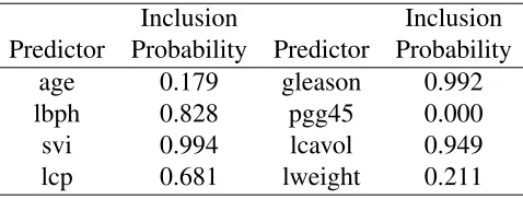
study . . . 44 Table 2.9 Marginal inclusion probabilities of predictors for Prostate cancer data . . . . 46

Table 3.1 Simulation results for AR(1) model based on 100 replications; figures in parentheses indicate standard errors . . . 71 Table 3.2 Simulation results for AR(4) model based on 100 replications; figures in

parentheses indicate standard errors . . . 73 Table 3.3 Simulation results for FGN model based on 100 replications; figures in

parentheses indicate standard errors . . . 75

(14)

LIST OF FIGURES

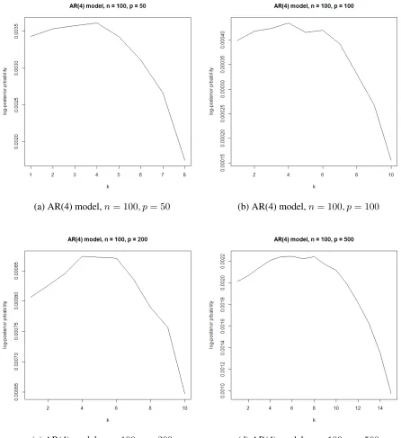
Figure 3.1 [Left] Structure of a banded precision matrix with shaded non-zero entries. [Right] The graphical model corresponding to a banded precision matrix of dimension 6 and banding parameter 3. . . 51 Figure 3.2 Figures showing log-posterior probabilities of graphs corresponding to

dif-ferent banding parametersk. The graphs are trimmed for larger values of

k as the log-posterior probabilities decay further. . . 70 Figure 4.1 Graphical structure of the median probability model selected by the Bayesian

graphical structure learning method. . . 113 Figure 4.2 Graphical structure corresponding to the subgraph corresponding to the

(15)

Chapter 1 Introduction

High-dimensional statistical inference has recently become one of the most important problems

in statistics, in which the number of unknown parameters pis much larger than the available sample sizen, that is, p n. Such kind of high dimensional problems include regression, classification, clustering, multiple testing, random matrices, and graphical models. This work

focuses on inference for high dimensional regression models including both parametric and

non-parametric mean functions, and large random matrices like precision (inverse covariance)

matrices using graphical models. We discuss some preliminaries on high dimensional

regres-sion and then introduce the concept of graphical models required for analysis of large matrices.

We introduce classical and Bayesian methods available for inference on large matrices. We

give a brief account of Bayesian asymptotics which we will be used in obtaining convergence

(16)

1.1 High dimensional regression models

Consider a linear regression model Yi = XiTβ +εi, i = 1, . . . , n. Here β = (β1, . . . , βp)T

is the vector of regression parameters and X = (X1, . . . , Xp)T is the set of p predictors for

the dependent variable Y. The random errors are εi iid∼ N(0, σ2). One of the main goals in this context is consistent estimation of the regression coefficients. As the dimensionp grows to infinity, the classical methods for estimation of the unknown parameters behave poorly. For

instance, the least square estimator is not uniquely defined and has high variability. In such

situations, we need to choose an effective set of predictors of dimension much smaller than

p, the problem better known as variable selection problem. Variable selection methods aim at identifying a set of predictors for which the coefficientsβj are non-zero. Efficient variable

selection methods help to improve accuracy in estimation, reduce computational complexity

and make the models more interpretable. In such cases, reasonable estimation is possible ifβ

is sparse in some sense. Generally, a condition like

logp× {sparsity(β)} n, (1.1)

depending on the type of sparsity specification onβwill allow reasonable estimation.

1.1.1 Classical variable selection

A number of variable selection and estimation procedures for linear regression models abound

the literature; see, for example Miller (2002) and George (2000). Most of these procedures use

the idea of penalization of the negative log-likelihood. Of these, one of the most significant and

widely used techniques is the Least Absolute Shrinkage and Selection Operator, or the lasso,

(17)

applicability in a variety of regression models. We briefly discuss the concept of lasso below.

The linear regression model above can be written in the matrix and vector notation as

Y =Xβ+ε, (1.2)

where Y is then ×1vector of responses, X is then ×pdesign matrix, β is the vector of regression parameters andεis then×1vector of random errors. The lasso estimator is defined as

ˆ

β(λ) = argmin_β kY −Xβk2

2+λkβk1

, (1.3)

wherekβk1 =

Pp

j=1|βj|andλ≥0is the penalty parameter. Forλ= 0, the solution becomes

the ordinary least square estimate. Depending on the choice ofλ, the lasso shrinks the least square solutions towards zero. The most important aspect of the lasso is that it produces exact

zero solutions for some components of the parameter, that is, for some j, βjˆ(λ) = 0, so that variable selection is automatically done. The tuning parameter λ may be chosen by cross-validation or using model selection criteria like the Akaike Information Criterion (AIC) or the

Bayesian Information Criterion (BIC). These techniques perform well for prediction purposes,

but a larger value of the penalty parameter is often necessary for effective variable selection

(B¨uhlmann and van de Geer, 2011). Consider the set of variables selected by the lasso for a

givenλ, given by

ˆ

S(λ) ={j: ˆβj 6= 0, j = 1, . . . , p}, (1.4)

(18)

the parameter space, it can be shown that forλ=λn n−1/2(logp)1/2,

P( ˆSλ =S0)→1, (1.5)

as n → ∞ (Meinshausen and B¨uhlmann, 2006). This result implies that the lasso proce-dure performs consistent variable selection under appropriate sparsity assumptions on the true

model.

Many other variable selection approaches are variations on this penalized regression theme

and typically differ from the lasso by varying the form of the penalty; see, for example, Breiman

(1995); Fan and Li (2001); Zou and Hastie (2005); Zou (2006); Bondell and Reich (2008);

Hwang et al. (2009) and so on.

In some situations, the underlying predictors form natural groupings, for example, sets

of dummy variables for factors, or in additive models where the effect of the predictors are

expanded in a basis. Yuan and Lin (2006) presented a variable selection technique, called the

group lasso in this context. Similar to the lasso, the group lasso is also a penalized least-squares

method that uses a special form of penalty, called the group-L1 penalty, to eliminate redundant

variables from the model simultaneously in a pre-specified groups of variables.

LetY be ann×1vector of responses,Xj is ann×mj matrix of variables associated with

thejth predictor (which may be fixed or random) andβj is anmj ×1vector of coefficients.

Then the group lasso minimizes

argmin_β

Y − g X

j=1

Xjβj

2

+λ g X

j=1

kβjk2, (1.6)

where β = (β1T, . . . ,βgT)T andg is the number of groups. For appropriate choices of the

(19)

1.1.2 Bayesian variable selection

One drawback of most classical variable selection methods is that they do not provide a

sure of model uncertainty and typically give one model as the best, without giving some

mea-surement of uncertainty for this estimated model. The exceptions to this are methods that

follow the Bayesian paradigm. They provide a measure of model uncertainty by computing

the posterior probabilities of models, which are typically estimated by the proportions of visits

to these models in the posterior draws from a Markov chain Monte Carlo (MCMC) simulation

(George and McCulloch, 1993). However, MCMC methods are computationally expensive

when a large number of variables are involved and it can be hard to assess convergence when

MCMC methods must traverse a space of differing dimensions. In fact, when the model

di-mension is quite high, most MCMC based methods break down.

Consider the linear regression set-up as in equation (1.2), and define thep-dimensional vec-torγ = (γ1, . . . , γp)T such thatγj = 1if Xj is included in the model andγj = 0otherwise.

LetXγ andβγ respectively denote the matrix of covariates and the vector of regression

coeffi-cients corresponding to the non-zero elements ofγ. In a Bayesian variable selection approach,

a prior distribution is assigned to all possible modelsγalong with prior distributions for the

un-known parametersβγ andσ2. Prior distributions are usually specified in a hierarchical fashion,

as

p(βγ,γ, σ2) =p(βγ |γ, σ2)p(γ)p(σ2). (1.7)

The marginal posterior distribution of a modelγis then given by

(20)

where

p(Y |γ) = Z

p(Y |βγ,γ, σ2)p(βγ, σ2 |γ)dβγdσ2. (1.9)

Posterior probabilities of models can be used to determine the model with highest posterior

probability. Barbieri and Berger (2004) showed that the median probability model, defined as

the collection of all variables whose marginal inclusion probabilities are at least1/2, has better prediction properties compared with the highest posterior probability model. In addition to

this, the posterior probabilities of various models can be used to perform Bayesian model

av-eraging (BMA), which incorporates model uncertainty and is typically preferred for prediction

purposes.

Choice of prior distribution on regression coefficients plays a vital role in model

assess-ment. In many instances, independent priors are put on the regression coefficients as a mixture

of two components conditioned onγ, given by

p(βj |γj) = (1−γj)p(0)(βj) +γjp(1)(βj). (1.10)

Mitchell and Beauchamp (1988) proposed the ‘spike and slab’ prior for βj by choosing the

priorsp(0)_(β

j) = 1l{0}(βj)andp(1)(βj) = 1l[−a,a](βj)/2a. Note that this prior has positive prior

probability forβj = 0so that variable selection can be done using model posterior probabilities.

George and McCulloch (1993) used a mixture prior for β given by p(0)(βj) = N(0, τj2) and p(1)(βj) = N(0, c2_jτ_j2). Here the constantτ_j2is chosen to be very small so that ifγj = 0, thenβj

has very negligible variance and may be dropped from the selected model. On the other hand,

the constantc2

j is chosen to be large, so that ifγj = 1,βj is included in the final model.

In most of the applications for variable selection, the dimensionpis large, and hence eval-uation of all2p _{possible models is not feasible. George and McCulloch (1993) applied a Gibbs}

(21)

search the model space (SSVS; also see George and McCulloch, 1997). A related MCMC

based approach is theMC3algorithm (Raftery et al., 1997) based on random-walk Metropolis sampler. Other stochastic search variable selection methods include the Laplace

approxima-tion based method by Yuan and Lin (2005) and the rescaled spike and slab prior proposed by

Ishwaran and Rao (2005).

Dependent priors on β are also used for variable selection. One of the most widely used

priors in this regard is Zellner’sg-prior (Zellner, 1986) given by

p(βγ |σ2, g)∼N(0, gσ2(XγTXγ)−1). (1.11)

The constant g is used to control the uncertainty in the prior relative to the variance of the observations around the mean, and the(X_γTXγ)−1 term provides a prior covariance structure

forβγ. The posterior model probabilities are analytically expressible in this case, and hence are

computationally simple. To resolve some inconsistencies arising from using a fixedg, Liang et al. (2008) used mixtures of Zellner’sg-prior, such as the Zellner-Siow Cauchy prior (Zellner and Siow, 1980) or the hyper-g prior (Liang et al., 2008).

Penalized regression methods in classical variable selection can also be viewed from the

Bayesian perspective. For instance, the lasso can be characterized as the posterior mode when

the regression parameters are assigned a common Laplace prior independent of the coefficients.

Park and Casella (2008) designed MCMC schemes for computing the posterior distribution by

representing the Laplace distribution as scale mixture of normals, and termed the resulting

procedure the Bayesian lasso. It may be noted that the Bayesian lasso does not incorporate any

sparsity unless it is complemented by an external thresholding procedure. Yuan and Lin (2005)

used the Laplace prior for the regression coefficients along with a point mass at zero, and

(22)

by expanding the prior times the likelihood around the posterior mode, which in this case is

identical with the lasso.

Similar to the lasso, the group lasso can be viewed as the posterior mode with respect to

some appropriate multivariate Laplace prior, where the grouping structure is induced by the

dependence in the components. Curtis et al. (2014) used such a kind of prior for variable

selection and developed a fast approximate method of evaluating posterior probabilities of

different models in the context of nonparametric additive regression. We shall extend their

technique for variable selection to cover generalized additive partial linear models.

1.2 Undirected graphical models

We first introduce some preliminary concept on graphs, and then proceed to the notion of

graphical models.

AnundirectedgraphGconsists of a finite non-empty setV ofppoints, called vertices, and a set of edgesE = {(i, j) ∈ V ×V;i < j}. Asubgraph G0 = (V0, E0)ofG = (V, E)is a graph such thatV0 ⊆V, E0 ={(i, j)∈V0×V0;i < j}.

In a graphical model, the vertex set V = {1, . . . , p} of a graph G corresponds to a p -dimensional random variable X = (X1, . . . , Xp)T ∼ P. The graph G equipped with the

probability distributionP is referred to as a graphical model(G, P). For an undirected graph, the graphical model is called an undirected graphical model. We shall consider all the related

concepts introduced henceforth for undirected graphical models.

1.2.1 Markov properties of a graphical model

(23)

Definition 1. The probability distributionP satisfies the pairwise Markov property with respect to an undirected graphGif for any distinct verticesjandksuch that(j, k)∈/ E,

Xj ⊥Xk |XV\{j,k}

A stronger version of the pairwise Markov property is the global Markov property which

we define below.

Definition 2. The probability distributionP satisfies the global Markov property with respect to an undirected graph Gif for disjoint subsets A, B, C such that C separates A andB, we have,

XA⊥XB |XC

Note that the global Markov property implies the pairwise Markov property. The two

become equivalent under some special cases.

Proposition 1. If the distribution P has a positive and continuous density with respect to a Lebesgue measure, then the pairwise and global Markov properties ofP are equivalent.

A Conditional Independence Graph (CIG) is a graphical model for which the pairwise

Markov property holds.

1.2.2 Gaussian graphical models

Consider a p-dimensional Gaussian random variable X = (X1, . . . , Xp)T ∼ Np(0,Σ). A

conditional independence graph with a Gaussian distribution on the random variables indexed

by the vertices of the graph is called a Gaussian graphical model (GGM). Due to Gaussian

(24)

of an edge is reflected in the zeroes of the precision matrixΩ=Σ−1 _{of the random variables.}

Thus we have,

(j, k)∈/ E ⇐⇒Xj ⊥Xk |XV\{j,k} ⇐⇒ωjk = 0, (1.12)

whereωjk is the (j, k)th element of Ω. Thus, the conditional independence of any two

com-ponents of the random variableX is reflected by a zero in the corresponding position of the

precision matrix.

1.3 Inference on large matrices

Estimating a covariance matrix or a precision matrix (inverse covariance matrix) is one of the

most important problems in multivariate analysis. Of special interest are situations where the

number of underlying variablespis much larger than the sample sizen. Situations like this are common in gene expression data, fMRI data and in several other modern applications. Special

care needs to be taken for tackling such high-dimensional scenarios. Conventional estimators

like the sample covariance matrix or maximum likelihood estimator behave poorly when the

dimensionality is much higher than the sample size.

1.3.1 Classical methods for estimating large matrices

Different regularization based methods have been proposed and developed in the recent years

for dealing with high-dimensional data. These include banding, thresholding, tapering and

penalization based methods to name a few; see, for example, Ledoit and Wolf (2004); Huang

et al. (2006); Yuan and Lin (2007); Bickel and Levina (2008a,b); Karoui (2008); Friedman et al.

(2008); Rothman et al. (2008); Lam and Fan (2009); Rothman et al. (2009); Cai et al. (2010,

(25)

sparse structure in the covariance or the precision matrix, as in Bickel and Levina (2008a),

where a rate of convergence was derived for the estimator obtained by “banding” the sample

covariance matrix, or by banding the Cholesky factor of the inverse sample covariance matrix,

as long asn−1_log_p_→₀_{. Cai et al. (2010) obtained the minimax rate under the operator norm}

and constructed a tapering estimator which attains the minimax rate over a smoothness class of

covariance matrices. Cai and Liu (2011) proposed an adaptive thresholding procedure. More

recently, Cai and Yuan (2012) introduced a data-driven block-thresholding estimator which is

shown to be optimally rate adaptive over some smoothness classes of covariance matrices.

For estimation of a sparse inverse covariance matrix, graphical models (Lauritzen, 1996)

provide an excellent tool, as the conditional dependency between the variables is captured by

means of an undirected graph; see Dobra et al. (2004); Meinshausen and B¨uhlmann (2006);

Yuan and Lin (2007); Friedman et al. (2008). There are several methods in the frequentist

literature for estimation of the precision matrix through graphical models. These methods

include minimization of the penalized log-likelihood of the data with a lasso type penalty on

the elements of the precision matrix. Several algorithms have been developed in the literature

to solve the above optimization problem, including coordinate descent based algorithm for the

lasso, which is popularly known as the graphical lasso (Meinshausen and B¨uhlmann, 2006;

Friedman et al., 2008; Banerjee et al., 2008; Yuan and Lin, 2007; Guo et al., 2011; Witten

et al., 2011). Other methods include the Sparse Permutation Invariant Covariance Estimator

(SPICE) as developed by Rothman et al. (2008).

1.3.2 Bayesian methods for estimating large matrices

There are only a few relevant work in Bayesian inference for such kind of problems. Ghosal

(26)

the dimensionp→ ∞, but restricting top n. Recently, Pati et al. (2012) considered sparse Bayesian factor models for dimensionality reduction in high dimensional problems and showed

consistency in theL2-operator norm (also known as the spectral norm) by using a point mass

mixture prior on the factor loadings, assuming such a factor model representation of the true

covariance matrix.

Bayesian methods for inference using graphical models have also been developed, as in

Roverato (2000); Atay-Kayis and Massam (2005); Letac and Massam (2007). For a complete

graph corresponding to the saturated model, clearly the Wishart distribution is the conjugate

prior for the precision matrixΩ. For an incomplete decomposable graph, a conjugate family of priors is given by theG-Wishart prior (Roverato, 2000). The equivalent prior on the covari-ance matrix is termed as the hyper inverse Wishart distribution in Dawid and Lauritzen (1993).

Letac and Massam (2007) introduced a more general family of conjugate priors for the

preci-sion matrix, known as theWPG-Wishart family of distributions, which also has the conjugacy

property. The properties of this family of distribution were further explored by Rajaratnam

et al. (2008), who also obtained expressions for Bayes estimators under different loss

func-tions. Wang (2012) developed a Bayesian version of the graphical lasso, putting Laplace priors

on the off-diagonal elements of the precision matrix and exponential priors on the diagonals.

Similar in lines with the Bayesian lasso (Park and Casella, 2008), the posterior mode in this

case coincides with the graphical lasso estimate. A block Gibbs sampler is also developed for

sampling from the resulting posterior distribution.

1.4 Asymptotics in Bayesian inference

In this section, we discuss and review the asymptotic properties of posterior distributions. We

(27)

experiments parametrized by a parameterθ, possibly of infinite dimension, taking values in a separable metric space. LetΠbe the prior distribution onθ and for data of sizendenoted by

X(n)_{, the posterior distribution is given by}_{Π(· |} _X(n)₎_{. The joint density of observations is}

denoted bypθ,n(X(n)). The posterior distribution is said to beconsistentat a givenθ0, if

Π(d(θ, θ0)> |X(n))→0 inP_θ(₀n)probability, (1.13)

asn → ∞for some distance metricdand any >0whenθ0is the true value of the parameter.

Consistency is almost guaranteed for finite-dimensional parameter spaces, if the support of

the prior is in the neighborhoods of the true parameter. But for infinite-dimensional spaces, this

alone is not sufficient to ensure posterior consistency. Some counterexamples in this context

were discussed in Freedman (1963), Diaconis and Freedman (1986), Kim and Lee (2001) and

James (2008). These examples show that more conditions are required on the prior to ensure

consistency.

If explicit forms of the posterior distribution is available, then posterior consistency results

may be proved using Chebychev-type inequalities. Examples of such include Bayesian survival

analysis problems where posterior conjugacy holds for priors described by an independent

in-crement process, and also in the case of posterior distributions arising from Dirichlet process

priors. Posterior consistency also holds for Bayesian estimation of a c.d.f, using tail-free

pri-ors. All of these involve much restrictive cases, and better approaches need to be exploited

for checking consistency in the general case. The theory by Schwartz (1965) is useful in this

respect, when the family of densities is dominated. The theory provides two sufficient

con-ditions required for consistency. The first condition is to construct strictly unbiased tests for

θ =θ0 against the alternativeθ∈B,B being the complement of a neighborhoodU ofθ0. The

(28)

exponentially fast. The second condition, known as Schwartz’s prior positivity condition, or

theKullback-Leibler propertyof the prior, requires thatΠ(θ:K(pθ0;pθ)< )>0for all >0,

whereK(pθ0;pθ) =

R

pθ0log(pθ0/pθ)dν is the Kullback-Leibler divergence between the two

densitiespθ0 andpθ (with respect to a dominating measureν). This condition is a crucial one

for establishing consistency.

However, the above procedure faces difficulties in infinite-dimensional spaces with stronger

topologies, unless the parameter space is compact. Ghosal et al. (1999) considered a technique

based on truncating the parameter space depending on the sample size. For this, they

consid-ered a sequence of subsets of the parameter space, called sieve, and show that by applying

Schwartz’s testing criterion on a carefully chosen sieve, posterior consistency can be obtained

by bounding the metric entropy of the sieve and the prior probability of the complement of the

sieve. A similar result under stronger condition using bracketing entropy was given by Barron

et al. (1999).

We now discuss convergence rates of posterior distributions, which is another important

aspect of Bayesian asymptotics. For a dataX(n)generated by a modelP_θ(n), a sequencen→0

is called theconvergence rate of the posterior distributionΠ(· |X(n)₎_{at the true parameter}_θ 0

with respect to a pseudo-metricd, if

Π(θ:d(θ, θ0)≥Mnn)→0 inP

(n)

θ0 probability, (1.14)

for any sequenceMn→ ∞.

The convergence rate in regular parametric families is well known to ben−1/2_{, whereas for}

infinite-dimensional models, the rate is generally slower thann−1/2_{. If the posterior converges}

at the raten, then there exists point estimator which converges to the true parameter at raten

(29)

be better than the minimax rate in a class, for which attaining the latter can be regarded as

the goal. Posterior convergence rate may be obtained in some situations using

Chebychev-type inequalities, in problems where the parameter space is equipped with the L2-norm and

explicit expressions for posterior mean and posterior variance are available. Also for

infinite-dimensional problems, convergence rate may be obtained by explicit calculations in situations

involving conjugate normal priors for normal mean. General results on obtaining posterior

convergence rates was given by Ghosal et al. (2000). We briefly summarize their idea here. For

i.i.d. observationsX1, . . . , Xn ∼p0, the posterior probability of the setB ={p:d(p, p0)≥n}

is expressed as a ratio

Π(θ ∈B |X1, . . . , Xn) = R

Bpθ,n(X1, . . . , Xn)/pθ0,n(X1, . . . , Xn)dΠ(θ)

R

pθ,n(X1, . . . , Xn)/pθ0,n(X1, . . . , Xn)dΠ(θ)

. (1.15)

Then, the desired convergence rate may be established if it can be shown that, (i) the numerator

is upper bounded bye−cn2n_{, where}c > 0_{can be chosen sufficiently large, and (ii) the}

denom-inator is lower bounded bye−bn2n. For satisfying the second assertion, the Kullback-Leibler

positivity condition in the consistency result is replaced by a stronger one given by

Π(B(p0, n))≥e−b1n

2

n_, _(1.16)

whereB(p0, n) ={p:K(p0;p)≤2n, V(p0;p)≤2n}, andV(p0;p) =

R

p0(log(p0/p))2. Thus

the prior distribution is required to have sufficient level of concentration around the true density

p0 in terms of the first and second moments of the log-likelihood ratio. Thisn is termed as

the prior concentration rate. For bounding the numerator of (1.15), the testing approach of

Schwartz (1965) is used. We find tests for the null hypothesisp = p0 against the alternative

(30)

Unless the parameter space is compact, such tests are constructed by the technique of sieves.

The sieve Pn is covered using balls of size ¯n/2 and the number of such balls need to be

controlled by the metric entropy condition

logN(¯n/2,Pn, d)≤c1n¯2n. (1.17)

In addition to this, we also need to ensure that the prior probability on the complement of

the sieve is exponentially small, that is,Π(Pc n) ≤ e

−c2n2n. The posterior convergence rate is

obtained by choosing the maximum of the prior concentration ratenand¯n. For obtaining the

minimax rate, the two rates need to match.

1.5 Notations

We now describe the notations to be used in this work. Bytn =O(δn)(respectively,o(δn)), we

mean thattn/δnis bounded (respectively,tn/δn →0asn → ∞). For a random sequenceXn, Xn=OP(δn)(respectively,Xn =oP(δn)) means thatP(|Xn| ≤M δn)→1for some constant M (respectively, P(|Xn| < δn) → 1for all > 0). For numerical sequencesrn andsn, by

rn sn(or,rn sn)we mean thatrn =o(sn), while bysn& rnwe mean thatrn=O(sn).

Byrn sn, we mean thatrn= O(sn)andsn =O(rn), whilern ∼snstands forrn/sn → 1.

The indicator function is denoted by1l.

We represent vectors in bold lowercase English or Greek letters. The components of

a vector are represented by the corresponding non-bold letters, that is, for x ∈ _Rp_, _x ₌ (x1, . . . , xp)T. We define the following norms for a vectorx∈ Rp: kxkr =

_Pp

j=1|xj|r 1/r

,

(31)

English or Greek letters, like A = ((aij)), where aij stands for the(i, j)th entry of A. The

identity matrix of order p will be denoted by Ip. If A is a symmetric p × p matrix, let eig₁(A) ≤ . . . ≤ eig_p(A) stand for its eigenvalues and let the trace of A be denoted by

tr(A). Viewing A as a vector in_Rp2

, we define Lr, 1 ≤ r < ∞ and L∞-norms on p×p

matrices as

kAkr = p X

i=1

p X

j=1

|aij|r !1/r

, 1≤r <∞, kAk∞ = max

1≤i,j≤p|aij|.

Note thatkAk2 =

p

tr(AT_A₎_{, the Frobenius norm. Viewing}_A_{an operator from}₍

Rp,k · kr)

to(_Rp_,_{k · k}

s), where1 ≤ r, s ≤ ∞, we can also define, kAk(r,s) = sup(kAxks:kxkr = 1).

We refer to the normk · k(r,r)as theLr-operator norm. This gives

kAk(1,1) = maxjP_i|aij|, kAk(∞,∞) = maxiP_j|aij|,

kAk(2,2) ={max(eigi(ATA): 1≤i≤p)}1/2,

and that for symmetric matrices, kAk(2,2) = max{|eigi(A)|: 1 ≤ i ≤ p}, and kAk(1,1) =

kAk(∞,∞). We state the following lemma involving relations between different matrix norms. Lemma 1. For symmetric matricesAandBof orderp, we have the following:

1. kAk(2,2) ≤ kAk(∞,∞)≤

√

pkAk(2,2); 2. kAk∞ ≤ kAk(2,2) ≤ kAk(∞,∞) ≤pkAk∞; 3. kAk(2,2) ≤ kAk2 ≤pkAk∞;

4. kABk2 ≤ kAk(2,2)kBk2, kABk2 ≤ kAk2kBk(2,2).

(32)

A, where0stands for the zero matrix.A1/2_{stands for the unique positive definite square root}

of a positive definite matrixA.

Sets are denoted in non-bold uppercase English letters. For a setT, we denote the cardi-nality, that is, the number of elements inT, by#T. We denote the submatrix of the matrixA

induced by the set T ⊂ {1,2, . . . , p}byAT, i.e., AT = ((aij:i, j ∈ T)). ByA−T1, we mean

the inverse(AT)−1 of the submatrixAT. For ap×pmatrixA= ((aij)), let(AT)0 = ((a∗ij))

denote ap-dimensional matrix such thata∗_ij =aij for(i, j)∈T ×T, and0otherwise. Also we denote the “banded” version ofAbyBk(A) = ((aij1l{|i−j| ≤k}))corresponding to banding parameter k, k < p. Finally, we define E(i,j) = ((1l{(i,j),(j,i)}(l, m))), which is a symmetric

matrix.

The Hellinger distance between two densities q1 and q2 is given by h(q1, q2) = k

√ q1 −

√ q2k2.

(33)

Chapter 2 Bayesian variable selection in generalized

additive partial linear models

2.1 Introduction

Linear models are widely used to analyze the relationship between any response variable with

relevant predictors of interest. If the response variable is discrete, a linear model is often

in-appropriate. Generalized linear models (GLM) (McCullagh and Nelder, 1983) provide useful

generalization of linear models which can handle various types of response variables including

discrete ones. In a GLM, the relationship between distribution of the response variable and the

predictors is expressed in terms of a linear functional form through a link function depending

on the distributional assumption of the underlying response. Typically these distributions are

assumed to belong to the exponential family, which includes a wide range of distributions

in-cluding binomial, Poisson and normal distributions. Regression modeling using GLMs can be

extended to generalized additive models (GAM), where the linear functional part in regression

(34)

pre-dictors (Hastie and Tibshirani, 1990; Wood, 2006). GAMs are especially useful in situations

when the relationship between the response variable and the predictors for a given link

func-tion is not linear. GAMs can be made further flexible by allowing a linear component for some

predictors which are presumed to have a strictly linear effect, and an additive structure for other

predictors. These models, known as generalized additive partial linear models (GAPLM), give

a natural extension of additive partial linear models (APLM) for discrete response variables.

GAPLMs incorporate more flexibility in the models by allowing both parametric and

non-parametric components, and particularly useful in situations where there is a prior knowledge

that some predictors can have a linear effect only, for example, binary predictors or dummy

indicator variables related to discrete predictors.

Statistical inference for GAPLMs have been well studied in the literature, with procedures

including kernel-based backfitting and local scoring (Buja et al., 1989) and marginal

integra-tion (Linton and Nielsen, 1995). Methods involving penalized regression splines (Marx and

Eilers, 1998; Ruppert et al., 2003; Wood, 2004) are also widely used in this regard, due to

computational simplicity and ease of implementation; see ‘gam’ and ‘mgcv’ package in R.

An important aspect in this regard is variable selection in these models. Variable

selec-tion in generalized linear models have been widely studied in the literature; for example, see

Raftery and Richardson (1993); Raftery (1996); Chen et al. (1999); Dellaportas and Forster

(1999); Meyer and Laud (2002); Ntzoufras et al. (2003); Wang and George (2007). Variable

selection methods for additive models have also been well studied; see Chen (1993);

Shiv-ely et al. (1999); Shi and Tsai (1999); Gustafson (2000); Wood et al. (2002); Avalos et al.

(2003); Lin and Zhang (2006); Belitz and Lang (2008); Meier et al. (2009); Ravikumar et al.

(2009); Reich et al. (2009); Huang et al. (2010); Marra and Wood (2011); Curtis et al. (2014).

The literature is quite sparse for variable selection in GAPLM. Wang et al. (2011) considered

(35)

APLMs has been studied much recently. Liu et al. (2011) developed a SCAD-based variable

selection procedure using a spline based approximation for the non-parametric components.

In contrast to a number of Bayesian methods for variable selection in additive models, to the

best of our knowledge, there is no Bayesian variable selection method for GAPLMs available

in the literature. Bayesian methods available in variable selection problems provide measures

of model uncertainty. However, in the high dimensional setting, Bayesian variable selection

methods are computationally expensive, since commonly used MCMC based procedures do

not scale well in high dimension. Moreover, even when such a procedure is implemented,

esti-mates of posterior probabilities from MCMC visits to different models can be extremely

unre-liable when the number of parameters is high. Curtis et al. (2014) developed a Bayesian

vari-able selection method in non-parametric additive regression models by approximating different

model posterior probabilities using Laplace approximation, thus avoiding any time-consuming

MCMC based procedures. In this chapter we extend the idea to GAPLMs, thus providing a

fast Bayesian variable selection technique for the same.

We expand each function in the non-parametric part of the model in a B-spline basis and put

a multivariate Laplace prior on the resulting coefficients. For predictors with a linear effect,

we put a univariate Laplace prior on each of the coefficients. The posterior mode of can be

identified as the group lasso for generalized linear models. We use the group lasso to

approx-imate different model posterior probabilities using Laplace approximation. The approxapprox-imate

probabilities are used to find the model with highest posterior probability and also the median

probability model. We compute relevant measures like specificity and sensitivity to evaluate

the model selection performance of the Bayesian method.

The chapter is organized as follows. In Section 2.2, we specify the model and discuss the

prior distributions on the coefficients. In the next section, we derive the form of the posterior

(36)

methods for selecting the penalty parameter for the group lasso. We also discuss some common

families of distributions used often in practice in the context of generalized linear models. In

Section 2.4, we discuss APLM as a special case of GAPLM. In Section 2.5, we evaluate the

performance of the proposed Bayesian method through simulation studies and also present

three real data analyses.

2.2 Model and prior specification

Consider a response variableY andp+spredictorsX = (X1, . . . , Xp)T,Z = (Z1, . . . , Zs)T.

The responseY follows an exponential family density of the formexp{a(η)y+b(η) +c(y)}, where a(η)and b(η)are continuously differentiable, with a(η)having a non-zero derivative. The mean of the distribution is given byµ = −b0_(η)/a0_(η) _≡ _ψ(η)_{, and} _ψ _{is called the link}

function. The inverse map,η = ψ−1_(µ) _{which represents the predictor in terms of the mean}

of the response variable, is called the inverse link function. The true relation between Y and

(X,Z)is assumed to follow a generalized additive partial linear model (GAPLM) given by

η =XTβ+ s X j=1

fj(Zj), (2.1)

where X consists of those predictors which have a strictly linear effect, including binary or

other categorical covariates, and those with non-linear effects are collected inZ. The functions

fj(·), j = 1, . . . , s, are arbitrary smooth functions corresponding to each predictor Zj, j = 1, . . . , s, such thatE(fj(Zj)) = 0.

(37)

of the functions in terms of a B-spline basis as

fj(Zj) = mj

X l=1

αjlBjl(Zj), j = 1, . . . , s, (2.2)

where Bjl(Zj) denotes the lth component of the B-spline basis vector for Zj. The number

of terms mj act as the tuning parameters, and can be selected by using cross-validation. Let m0 =

Ps

j=1mj. Thus, the model in (2.1) can be written as

η=XTβ+ s X j=1 mj X l=1

αj,lBj,l(Zj). (2.3)

Considernindependent observationsY1, . . . , Yn with corresponding predictor variables given

byXi,Zi, 1≤ i ≤n and link functionsη = (η1, . . . , ηn)T. The above model can be written

in matrix-vector notation as

η =_Xβ+_Zα, (2.4)

where X n×p =         

X11 · · · X1p X21 · · · X2p

..

. . .. ...

Xn1 · · · Xnp          , (2.5) and, Z n×m0 =         

B11(Z11) · · · B1m1(Z11) · · · Bs1(Z1s) · · · Bsms(Z1s)

B11(Z21) · · · B1m1(Z21) · · · Bs1(Z2s) · · · Bsms(Z2s)

..

. . .. ... . .. ... . .. ...

B11(Zn1) · · · B1m1(Zn1) · · · Zs1(Zns) · · · Bsms(Zns)

(38)

We denote then×(p+m0)matrix of covariates as

Ψ n×(p+m0)

= (_X:_Z). (2.7)

The vector of co-efficients is(βT

p×1

, αT

m0×1

)T, where

β

p×1

= (β1, . . . , βp)T, (2.8)

and,

α

m0×1

= (αT₁

m1×1

, . . . , αT_s

ms×1

)T = (α11, . . . , α1m1, . . . , αs1, . . . , αsms)

T

. (2.9)

We assume that the true underlying model is actually sparse, and hence we are interested

in performing variable selection. We define the indicator vector

γ

(p+s)×1

= (γ₁X, . . . , γ_pX, γ₁Z, . . . , γ_sZ)T,

where

γ_jX =       

1, ifXj is in the model, 1≤j ≤p, 0, otherwise

γ_jZ =       

1, ifZj is in the model, 1≤j ≤s, 0, otherwise.

We denote the vector of co-efficients selected byγas(βT

γ,αTγ)T and the corresponding matrix

of covariates asΨγ = (Xγ,Zγ).

(39)

degenerate at0or has a Laplace density, depending onγX

j = 0orγjX = 1respectively, that is,

p(βj |γ) = (1−γjX)1l{0}(βj) +γjX λ

2exp{−λ|βj|}. (2.10)

For the co-efficients corresponding toZj, given byαj, 1≤j ≤s, we have point-mass at0

corresponding toγZ

j = 0and a multivariate Laplace density corresponding toγjZ = 1, so that

the prior density ofαj givenγ, denoted byp(αj |γ)is given by,

p(αj|γ) = (1−γjZ)1l{0}(αj) +γjZ

Γ(mj/2) 2πmj/2Γ(m

j) λmj

j exp{−λjkαjk}; (2.11)

here λ and λj, j = 1, . . . , s, act as the tuning parameters for the different coefficients. The

motivation behind the above choice of priors is to get the group lasso solution as the posterior

mode corresponding to the likelihood of the response variable. In the R package for the group

lasso, the tuning parameter is of the form λ√df, where df is the degrees of freedom of the corresponding predictor. Hence we take the tuning parameters to beλ andλj = λ

√

mj, j = 1, . . . , s, for the linear and the non-linear predictors respectively.

For a binary vector γ, the number of 1’s inγis denoted by|γ|. The prior on the variable selection indicatorγ is given by

p(γ)∝det(_XT_γ_Xγ)det(Kγ)q|γ|(1−q)(p+s)−|γ|, (2.12)

where q ∈ (0,1) and Kγ is formed by Kendall’s tau coefficients of the variables inγ with

non-linear effect, that is,Kγ = ((τ(Zj, Zl):γjZ, γlZ = 1)), where

τ(Zj, Zl) = 1 n

2

X X i<i0

(40)

is the Kendall’s tau-coefficient between two variablesZj andZl. The factordet(XTγXγ)

down-weights models with variable combinations having near linear dependence in the linear part,

whiledet(Kγ)downweights variable combinations with high degree of monotone associations

in the non-linear part. The following result shows that the matrixK = ((τ(Zj, Zl))), and hence

all submatricesKγ, are non-negative definite. Therefore use of the factordet(Kγ)is justified

in the specification of model prior probabilities.

Lemma 2. The matrixK = ((τ(Zj, Zl)))is always non-negative definite.

Proof. By definition of Kendall’s tau coefficient, the(j, l)th_{element of}_K _{is given by}

τ(Zj, Zl) = Pn

i=1

Pn

i0₌_i₊₁sign(Zij −Zi0_j)sign(Z_il−Z_i0_l)

n 2 = Pn i=1 Pn

i0₌₁sign(Zij −Zi0_j)sign(Z_il−Z_i0_l)

n(n−1) ,

j, l = 1,2, . . . , s,since sign(0) = 0. Therefore we need to show that for anya1, . . . , as, s X j=1 s X l=1 ajal n X i=1 n X i=1

sign(Zij −Zi0j)sign(Zil−Zi0l)≥0.

The expression is equal to

n X i=1 n X i=1 s X j=1

ajsign(Zij −Zi0_j)

! _s X

l=1

alsign(Zil−Zi0_l)

! = n X i=1 n X i0₌₁

s X

j=1

ajsign(Zij −Zi0_j)

!2 ≥0,

(41)

2.3 Posterior computation

The log likelihood of the parameters is given by

l(β,α;Y) = n X

i=1

{a(ηi)Yi+b(ηi) +c(Yi)}. (2.13)

Thus, the joint posterior densityp(βγ,αγ,γ | Y)forβγ,αγ andγ, givenY is proportional

to

p(Y|βγ,αγ,γ)p(βγ,αγ|γ)p(γ)

= (1−q)p+sdet(_XT_γ_Xγ)det(Kγ)

q 2(1−q)

|γ| 

Y {j:γZ

j=1}

Γ(mj/2)λmj

πmj/2Γ(m

j)   ×exp   

l(βγ,αγ;Y)−λ

X {j:γX

j =1}

|βj| −λj X {j:γZ

j=1}

kαjk   

. (2.14)

The marginal posterior probability for modelγ can be obtained by integrating outβγ and

αγ, that is,

p(γ|Y)∝C1(Y)C2(γ)

Z

Rmγ

exp{−h(βγ,αγ)}dβγdαγ, (2.15)

with

mγ =|γX|+

X {j:γZ

j=1}

mj,

C1(Y) = (1−q)p+s,

C2(γ) = det(XTγXγ)det(Kγ)

q 2(1−q)

|γ| λmγ

 

Y {j:γZ

j=1}

Γ(mj/2) πmj/2Γ(m

j)  ,

h(βγ,αγ) = −l(βγ,αγ;Y) +λ

X {j:γX

j =1}

|βj|+λj X {j:γZ

j=1}

kαjk.

(42)

The integral in (2.15) can be approximated using the Laplace’s approximation. Let(βT∗

γ ,αT

∗

γ )T

denote the group lasso solution, that is,

(β_γT∗,αT_γ∗)T = argmin

βγ,αγ

h(βγ,αγ). (2.17)

Putu = (uT

β,uTα) = (βγT,αTγ)T −(βT

∗

γ ,αT

∗

γ )T. Substituting this quantity into (2.15) gives

the expression

C1(Y)C2(γ) exp

−h(β_γ∗,α∗_γ) Z

Rmγ

exp{−f(u)}du, (2.18)

where,

f(u) = −{l(uβ +βγ∗,uα+α∗γ;Y)−l(β

∗

γ,α

∗

γ;Y)}

+λ X {j:γ_jX=1}

{|uβ,j +βj∗| − |β ∗ j|} +λj

X {j:γZ

j=1}

{kuα,j+α∗jk − kα ∗

jk}. (2.19)

Clearlyf(u)is minimized atu =0by definition. For the Laplace approximation we need to compute the Hessian of the functionf(u). We have,

∂l(uβ +βγ∗,uα+α∗γ;Y)

∂u =

∂ ∂u

n X

i=1

{a(ηi)Yi+b(ηi) +c(Yi)}

= n X

i=1

a0(ηi)

∂ηi ∂uYi+b

0 (ηi)

∂ηi ∂u = n X i=1

(43)

Ψibeing theithrow ofΨ. Differentiating the above expression again gives,

∂2_l(_u

β +βγ∗,uα+α∗γ;Y)

∂u∂uT =

n X

i=1

{a00(ηi)Yi+b00(ηi)}ΨTi Ψi. (2.20)

Atu =0, we have,

∂2_f₍_u₎

∂u∂uT

u=0

=− n X

i=1

{a00(ηi)Yi+b00(ηi)}ΨTi Ψi+λAγ, (2.21)

where themγ ×mγ matrixAγ is given by

Aγ =

  

O O

O AZ_γ

 

, (2.22)

Ostands for a zero matrix of appropriate order, andAZ

γ is given by

        

D1 O12 · · · O1t

O21 D2 · · · O2t

..

. ... . .. ...

Ot1 Ot2 · · · Dt          , (2.23)

where Dj = √ mj −α ∗ jα ∗T j

kα∗

jk3 +

I_mj−1

kα∗

jk

, j = 1, . . . , t(= |γZ_|)_{, and} _O

ij is the zero matrix

corresponding to the variables in theith row andjth column selected byγZ_.

(44)

which gives

p(γ|Y) ∝ C1(Y)C2(γ) exp

−h(β_γ∗,α∗_γ) × Z ∞ −∞ · · · Z ∞ −∞

exp{−f(u)}du

≈ C1(Y)C2(γ) exp

−h(β_γ∗,α∗_γ) ×exp{−f(0)}(2π)mγ/2

∂2_f₍₀₎

∂u∂uT

−1/2

.

The accuracy of the approximation is controlled by the dimension and the posterior

conver-gence rate. Substituting (2.21) in the above quantity, the marginal posterior probabilityp(γ|Y)

forγ is approximately proportional to

Q(γ|Y) = C1(Y)C2(γ) exp

−h(β_γ∗,α∗_γ) ×(2π)mγ/2

− n X i=1

{a00(ηi)Yi+b00(ηi)}ΨTi Ψi+λAγ

−1/2

. (2.24)

The approximation above is valid only for regular models, that is, models indicated byγ

for which the functionf(u)is differentiable atu=0. This holds only if the group lasso solu-tion for all the coefficients corresponding to the predictors included in the model as indicated

byγ are non-zero. If the group lasso solution is zero for a subset of variables already in the

model, then the corresponding model is termed as a non-regular model, and posterior

proba-bility cannot be approximated using the Laplace approximation. This issue of non-regularity

also arises in variable selection for linear models and non-parametric additive regression

mod-els; see Yuan and Lin (2005) and Curtis et al. (2014). The corresponding regular model for a

non-regular model is obtained by excluding the variables for which the group lasso solution is

(45)

Therefore it suffices to compute the model posterior probabilities of the regular models only

at least, if one wants to obtain the maximum posterior probability model. The approximate

posterior probabilities may be re-normalized taking only the regular models into account.

2.3.1 Estimation of

λ

The joint density of the response and the regression coefficient vector given the other model

parameters is given by

p(Y,βγ,αγ |γ, λ) =

1 2

|γ| λmγ

 

Y {j:γZ

j=1}

Γ(mj/2) πmj/2Γ(m

j)  

×exp{−h(βγ,αγ)}. (2.25)

Integrating outβγ andαγ, and using Laplace approximation as before, we get,

p(Y |γ, λ) ≈ 2−(2|γ|−mγ)/2_π|γX|_λmγ

×  

Y {j:γZ

j=1}

Γ(mj/2) Γ(mj)

 exp

−h(β_γ∗,α∗_γ)

× − n X i=1

−1/2

. (2.26)

Similar to the penalized maximum likelihood criterion as in Curtis et al. (2014), we can

(46)

loga-rithm of (2.26) gives,

r(λ) = (2|γ| −mγ) log 2−2|γX|logπ−2mγlogλ

−2 X

{j:γZ₌₁_}

{log Γ(mj/2)−log Γ(mj)}+ 2h(βγ∗,α

∗

γ)

+ log

− n X

i=1

. (2.27)

We estimateλby minimizing

r(λ) +mγˆλlogn. (2.28)

2.3.2 Examples of GAPLM

The expression for the approximate posterior probabilities of various models can be derived

explicitly for a given exponential family of distributions and the corresponding link function.

We discuss some of the densities which are widely used in this context and derive the form of

the Hessian required for the Laplace approximation of the posterior probabilities.

1. Logistic regression: The mean of the distribution is µ = exp(η)/(1 + exp(η)), and the response isY ∈ {0,1}. The likelihood is given by exp{ηy−log(1 + exp(η))}, so that

a(η) = η, b(η) = −log(1 + exp(η)). Thus, the expression of the Hessian as in (2.21) becomes,

∂2f(u) ∂u∂uT

u=0

= n X

i=1

exp(ηi) (1 + exp(ηi))2

ΨT_i Ψi +λAγ. (2.29)

(47)

Thus, expression (2.21) gives,

∂2_f(_u₎

∂u∂uT

u=0

= n X

i=1

exp(ηi)ΨTiΨi+λAγ. (2.30)

3. Probit regression: The mean of the distribution is given by the distribution function of

a standard normal distribution, that is, µ = Φ(η), and the response isY ∈ {0,1}. The likelihood is given by

exp

ylog

Φ(η) 1−Φ(η)

+ log(1−Φ(η))

.

Thus, a(η) = log(Φ(η)/(1−Φ(η))), b(η) = log(1−Φ(η)). The expression for (2.21) can be obtained by evaluating the second derivatives ofa(η)andb(η), given by

a00(η) = Φ

00_(η)Φ(η)₋_(Φ0_(η))2

(Φ(η))2 +

Φ00(η)(1−Φ(η)) + (Φ0(η))2

(1−Φ(η))2 ,

b00(η) = −Φ

00_(η)(1₋_{Φ(η)) + (Φ}0_(η))2

(1−Φ(η))2 . (2.31)

4. Exponential regression: For an exponential regression with exponential link, the mean

of the distribution isµ= exp(η), and responseY ∈ (0,∞). The likelihood is given by

exp(−exp(−η)y−η), so thata(η) = −exp(−η), b(η) = −η. Thus, the expression of (2.21) is given by

∂2_f(_u₎

∂u∂uT

u=0

= n X

i=1

{exp(−ηi)Yi}ΨTi Ψi+λAγ. (2.32)

5. Normal linear regression: For the normal linear regression set-up, we have the special

Bayesian Inference for High Dimensional Models: Convergence Properties and Computational Issues.

ABSTRACT

DEDICATION

BIOGRAPHY

ACKNOWLEDGEMENTS

TABLE OF CONTENTS

LIST OF TABLES

LIST OF FIGURES

Chapter 1

Introduction

1.1

High dimensional regression models

1.1.1

Classical variable selection

1.1.2

Bayesian variable selection

1.2

Undirected graphical models

1.2.1

Markov properties of a graphical model

1.2.2

Gaussian graphical models

1.3

Inference on large matrices

1.3.1

Classical methods for estimating large matrices

1.3.2

Bayesian methods for estimating large matrices

1.4

Asymptotics in Bayesian inference

1.5

Notations

Chapter 2

Bayesian variable selection in generalized

additive partial linear models

2.1

Introduction

2.2

Model and prior specification

2.3

Posterior computation

2.3.1

Estimation of

λ

2.3.2

Examples of GAPLM