On efficient Bayesian inference for models with stochastic volatility

(1)

Kent Academic Repository

Full text document (pdf)

Copyright & reuse

Content in the Kent Academic Repository is made available for research purposes. Unless otherwise stated all content is protected by copyright and in the absence of an open licence (eg Creative Commons), permissions for further reuse of content should be sought from the publisher, author or other copyright holder.

Versions of research

The version in the Kent Academic Repository may differ from the final published version.

Users are advised to check http://kar.kent.ac.uk for the status of the paper. Users should always cite the published version of record.

Enquiries

For any further enquiries regarding the licence status of this document, please contact: [email protected]

If you believe this document infringes copyright then please contact the KAR admin team with the take-down information provided at http://kar.kent.ac.uk/contact.html

Citation for published version

Griffin, Jim E. and Sakaria, Dhirendra Kumar (2016) On efficient Bayesian inference for models

with stochastic volatility. Econometrics and Statistics, 3 . pp. 23-33. ISSN 2452-3062.

DOI

https://doi.org/10.1016/j.ecosta.2016.08.002

Link to record in KAR

http://kar.kent.ac.uk/58710/

Document Version

Author's Accepted Manuscript

(2)

On efficient Bayesian inference for models with

stochastic volatility

D. K. Sakaria and J. E. Griffin

∗

Abstract

An efficient method for Bayesian inference in stochastic volatility models uses a linear state space representation to define a Gibbs sampler in which the volatili-ties are jointly updated. This method involves the choice of an offset parameter and we illustrate how its choice can have an important effect on the posterior inference. A Metropolis-Hastings algorithm is developed to robustify this approach to choice of the offset parameter. The method is illustrated on simulated data with known parameters, the daily log returns of the Eurostoxx index and a Bayesian vector au-toregressive model with stochastic volatility.

Keywords: Stochastic volatility; Bayesian methods; Markov chain Monte Carlo; Mix-ture offset representation.

∗_{Corresponding author: Professor Jim Griffin, School of Mathematics, Statistics and Actuarial Science,} University of Kent, Canterbury, CT2 7NF, U.K. (Email: [email protected])

(3)

1 Introduction

It is known that the volatility of many economic variables vary over time. Initial work on time-varying volatility often considered asset price returns. Over the long term, the volatility of equity returns may appear to be stable but usually there are periods of high volatility and calm market periods when the volatility may be low (Enders, 2004). Several approaches have been developed to model this time-varying volatility. In ARCH and GARCH models (Engle, 1982; Bollerslev, 1986), the volatility is modeled as a function of the lagged values of the asset returns and the volatility. Alternatively, stochastic volatility models assume that the volatility follows a known stochastic process such as an AR process for the logarithm of volatility (seee.g. Har-vey and Shephard, 1996).

In this paper, we will concentrate on the Bayesian estimation of stochastic volatil-ity models (seee.g.Jacquier et al., 1994; Kim et al., 1998; Chib et al., 2002). The asset returns may be expressed as function of past returns or other economic variables and the log volatility is modeled as a separate AR process. A simple stochastic volatility model assumes thatyt, the log return at timet, can be expressed as

yt=eht/2νt, t= 1, . . . , T (1)

ht=µ+φ(ht−1−µ) +σηηt.

where νt andηt are independent error terms for which νt i.i.d.∼ N(0,1)and ηt i.i.d.∼

N(0,1), andhtis the log volatility at timet. The model assumes that the log volatility

htfollows an AR(1) process with parametersµ,φ, andση.

Bayesian inference is complicated since this is a non-linear state space model. Several Markov chain Monte Carlo (MCMC) methods have been developed to sam-ple this class of models. Jacquier et al. (1994) used one-at-a-time updating ofhtwith

(4)

often criticised for higly correlated samples). Samplers which update a block ofht’s

often lead to better mixing. For example, Jensen and Maheu (2014) propose to up-date a block ofhtin an asymmetric, nonparametric stochastic volatility model.

The model (1) can be expressed in linear state space form for ht using

trans-formed datalogy_t2 =ht+ logνt2. Kim et al. (1998) (KSC) approximate the

distribu-tion oflogν_t2using a normal mixture distribution leading to a Gaussian linear state space form forhtconditional on the mixture states for each observation. This allows

the volatilitiesh1, . . . , hT to be updated using Forward Filtering Backward Sampling

(FFBS) techniques (Carter and Kohn, 1994; Fr ¨uhwirth-Schnatter, 1994). In order to make the approximation robust for small values ofyt, a small offset parameter cis

used andlog(y2

t +c) is used in place oflogyt2 as the transformed data. This leads

to samples from an approximate posterior distribution for the parameters of the SV model andh1, . . . , hT. KSC suggest an importance sampling scheme for estimating

posterior quantities using the approximate posterior as the importance sampling distribution. However, as with any importance sampler, results can become biased if the importance sampling distribution (the approximation) is sufficiently different to the actual posterior distribution. This can be the case ifcis poorly chosen. The ap-proach has been developed in various directions. Chib et al. (2002) consider models with Student-t distributed innovation, exogeneous variables and jumps in obser-vations. Omori and Watanabe (2008) consider an asymmetric stochastic volatility model and allow correlation between the returns and the volatility which allows the modelling fo the leverage effect. A multivariate normal approximation is used to express the model in a linear state space form with Gaussian errors. Results show a better performance compared to a single move sampler. More recently, Kastner and Fr ¨uhwirth-Schnatter (2014) developed centring methods.

(5)

mod-els. For example, Belmonte et al. (2013) consider dynamic regression models with stochastic volatility

yt=Xtβt+eht/2νt, t= 1, . . . , T (2)

or Clark (2012) builds a vector autoregressive model with stochastic volatility, which will be further considered in this paper. Let ytbe a (p×1)-dimensional vector of

economics variables andxtbe a(q×1)-dimensional vector of deterministic variables

measured at timet. The data modelled as

Π(L)(yt−Ψxt) =ǫt (3)

whereΨis a(p×q)-dimensional vector of coefficients,Π(L) =Ip−Ψ1L−Ψ2L2. . .ΨkLk

is a lag polynomial andνtare independent errors. The errorsǫtare modelled using

a factor stochastic volatility model. LetAbe a lower triangular matrix with 1’s on the diagonal then

ǫt=A−1Λ0t.5νt, νt∼N(0, Ip),

Λt=diag(eh1,t, eh2,t, . . . ehp,t),

hi,t) =hi,t−1+ση,iηi,t, ηi,t iid∼ N(0,1) ∀i= 1,2, . . . , p.

Bayesian inference is made using a Gibbs sampler and the volatilities are updated using the KSC method in the approximate model (i.e.usingr⋆

t = log((yt−Xtβt)2+c)

for the dynamic regression model or r⋆

t = AΨ(L)(yt−Ψxt) +cfor the vector

au-toregression model) but other parameters (such asβt) are updated using the correct

(rather than the approximate) stochastic volatity model. Although, this seems to have little effect on inference, the Gibbs sampler is not properly specified. In addi-tion, in these models, the effect ofcis harder to understand since the scale ofr⋆

t can

(6)

This paper makes two main contributions. Firstly, we develop an MCMC frame-work for sampling from the posterior distribution of the SV model (rather than an approximation to the SV model) using the KSC method as a proposal in a Metropolis-Hastings step for updating the volatilities. Secondly, we introduce a method for specifying the offset parameter using standardisation that robustifies the MCMC al-gorithm to the scale of the data.

The paper initially considers the problem of sampling the time-varying volatili-ties in the stochastic volatility model in (1) and considers more complicated models in the examples. The remainder of the paper is organised as follows. Section 2 de-scribes the Kim et al. (1998) method to linearise the log volatility model and the difficulty of using an appropriate value of the offset parametercis highlighted. In section 3, a standardisation method is introduced and a Metropolis-Hastings (M-H) step is described to propose volatility parameterh1, . . . , hT using Forward Filtering

Backward Sampling (FFBS). Results using simulated data, Eurostoxx daily log re-turns and a vector autoregressive model with stochastic volatility are discussed in section 4. Section 5 concludes.

2 Linear state space method

In this section, we review the sampling method of KSC and illustrate the effect of choosing c. KSC suggest transforming the observations in the SV model in (1) so that

logy_t2=ht+logνt2, (4)

which is now linear in ht. The error term logνt2 has a logχ21 density, which they

show can be accurately approximated by a normal mixture distribution. To make the method robust for small or zero values ofyt, a small offset parametercis used

(7)

(Fuller, 2009) so that y_t2 is replaced by y_t⋆ = y2_t +c. This leads to the following representation of the model in (4),

logy_t∗=ht+logνt2 (5)

KSC suggest approximating the distribution ofzt = logνt2, which is thelogχ21

dis-tribution, by the density

p(zt) =

7

X i=1

qifN(zt|mi−1.2704, v2i)

wherefN(x|µ, σ2)is the normal density with meanµand varianceσ2. Introducing

a mixture state indicatorstfort= 1, . . . , T allows the model to be written in a linear

state space form as

logy_t∗=ht+mst−1.2704 +vstǫt, (6)

ht=µ+φ(ht−1−µ) +σηηt,

whereǫt andνt are independent for whichνt i.i.d.∼ N(0,1)andηt i.i.d.∼ N(0,1), and

p(st = i) = qi. This allows a Gibbs sampler to be defined where the parameters

of the SV model can be updated from their full conditional distributions and the Gaussian, linear state space form in (6) allowed KSC to block sample the volatility parameterh = (h1, h2, . . . , hT) using the simulation signal smoother (De Jong and

Shephard, 1995). The method samples from an approximate posterior distribution and KSC describe how an importance sampler, with the approximation employed as importance sampling distribution, can be used to estimate posterior quantities of interest.

The choice of ccan have a large effect on the inferences. Kim et al. (1998) use

c = 0.001 for the Mixture Offset parameter, but state that “it is possible to let c

(8)

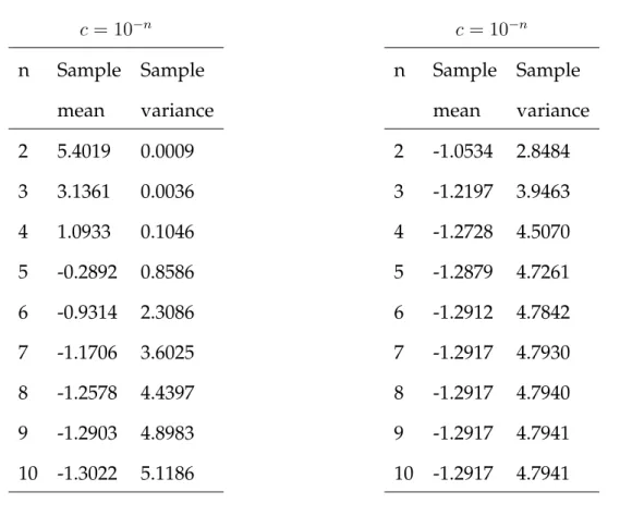
c= 10−n n Sample Sample mean variance 2 5.4019 0.0009 3 3.1361 0.0036 4 1.0933 0.1046 5 -0.2892 0.8586 6 -0.9314 2.3086 7 -1.1706 3.6025 8 -1.2578 4.4397 9 -1.2903 4.8983 10 -1.3022 5.1186 c= 10−n n Sample Sample mean variance 2 -1.0534 2.8484 3 -1.2197 3.9463 4 -1.2728 4.5070 5 -1.2879 4.7261 6 -1.2912 4.7842 7 -1.2917 4.7930 8 -1.2917 4.7940 9 -1.2917 4.7941 10 -1.2917 4.7941

Table 1: Sample mean and variance of log(y2_t +c)−htwhen his simulated using µ =

−10, φ= 0.95, σ_η2 = 0.012_{(left hand table) and when}_y

tis simulated directly from N(0,1), using different values of the offset parameterc.

using the SV model in (1) with µ = −10, φ = 0.95 and ση = 0.01. The sample

mean and sample variance oflog(y2

t +c)−htfor 1500 generated values are shown

in Table 1. Since the data is generated, it follows that logy_t2 −ht follows alog(χ21)

distribution whose mean is -1.2704 and whose variance is 4.93. Difference between these values of the mean and variance oflog(y2

t +c)−htshows the effect ofc. The

sample mean and variance are only close to the true values whencis smaller than 10−9. For larger values ofc, the sample mean is too large and the sample variance is too small. The value chosen by KSC works well if the log returns are on a unit scale but works badly in this case whenµ=−10.

(9)

The simulation results suggest that we can only choose a single value ofcfor all data if we can scale the data appropriately. In more complicated models, for example in a regression setting with stochastic volatility whereytis modelled as a function of

other variables, the residuals could depend on the current values of the parameters in the sampler. In this case, it would be difficult to set one value ofcwhich works with different parameter values. A scaling approach will be developed in Section 3 where we will re-scaleytto a variable with unit variance. To understand the effect of

con data with a unit variance we simulated 1500 data points from a standard normal distribution and calculated the sample mean and sample variance oflog(y_t2+c). The results in Table 1 show thatcneeds to be near10−3for the sample mean and sample variance to be near to the values withoutc.

3 Standardisation approach and its MCMC

sam-pler

The results in the previous section show that the value of the offset parameterccan have a strong influence on the shape of the distribution oflog(y_t2+c). Our method is based on the following idea. The model in (1) can be expressed asνt = yte−ht/2

whereνt ∼N(0,1)and so we can choose a single value ofcwhich does not have a

strong influence onlog(ν2

t +c) = log yt2e−ht+c

= log(y2

t+ceht)−ht. This suggests

the following standardised approximating model log(y_t2+ceht_{) =}_h

t+logνt2, (7)

The approach of KSC cannot be directly applied using this representation since it is no longer a linear state space model forht. This can be used to define alternative

(10)

offset parameterisations by replacing eht _{be an estimator which would allow the}

standard KSC method to be used. For example, one anonymous referee suggested using y∗_t =      log y2_t +cvar(y) yt= 0 log y2_t +c y_t2 yt6= 0 . (8)

However, it is hard to see how this can be easily implemented in more complicated model such as (2) or (3) where KSC is used on a residual rather than observed data. Our approach defines an MCMC sampler for the posterior distribution using the non-linear parameterisation in (1). The approximating model in (7) is used to de-fine a proposal forh1, . . . , hT, which can be sampled using FFBS, in a

Metropolis-Hastings step. In models such as (2), this scheme allows all model parameters to be correctly sampled using the non-linear parameterisation of the SV model.

To describe the MCMC sampling scheme, we will denote θ = {µ, φ, ση} and

h= (h1, . . . , hT)and so the joint posterior density forhandθis given by

p(h, θ|y) = p(y|h, θ)p(h|θ)p(θ)

p(y) .

To allow us to use FFBS to updateh, we use an augmented version of the posterior distribution for the non-linear parameterisation

(11)

and sampling from pq will lead to draw for θ andh from the posterior using the

non-linear parameterisation. An MCMC sampling scheme is run withpqas the

tar-get distribution. The parameters θ are updated from pq(θ|y, h) followed by s

up-dated frompq(s|θ, y, h)and, finally,hupdated frompq(h|θ, y, s)using a

Metropolis-Hastings step where the proposal arises from FFBS. The full details of the scheme are given below with the following priors: p(µ) ∝ 1, π(φ) ∝ 1+₂φa−11−₂φb−1,

σ_η−2 ∼Gaσr

2 ,S

σ

2

where Ga(a, b)represents a gamma distribution with meana/b

and variancea/b2_.

Samplingµ

The full conditional distribution ofµis N(ˆµ, σ2_µ)where ˆ µ=σ_µ2 (1−φ 2₎ σ2 η h1+ (1−φ) σ2 η t=T−1 X t=1 (ht+1−φht) ! , and σ2_µ=σ_η2 (T −1)(1−φ)2+ (1−φ2)−1. Samplingφ

The full conditional density forφis proportional toπ(φ)p(y|h, µ, φ, σ2

η).We update

this parameter using Metropolis-Hastings random walk whose proposal distribu-tion is a normal truncated to (−1,1)whose mean is the previous value of φ. The variance of the proposal is tuned using an Adaptive Metropolis-Hastings method (Atchade and Rosenthal, 2005) to get an acceptance rate of 23.4%.

(12)

Samplingσ_η2

The full conditional distribution ofσ−2

η is Ga(a, b)where a= T+σr 2 and b= Sσ+ (h1−µ) 2₍₁₋_φ2_{) +}Pt=T−1 t=1 ((ht+1−µ)−φ(ht−µ))2 2 . Samplings

The full conditional distribution ofsisg(s|h, θ, y)and sos1, . . . , sT are conditionally

independent withstsampled from the discrete distribution

pq(st=i|h, θ, y) = qip˜(log y2t +ceht)|ht, θ, st=i Pj=7 j=1qjp˜ log(y2t +ceht)|ht, θ, st=j . Samplingh

The full conditional density for h is proportional top(y|h, θ)p(h|θ)g(s|h, θ, y). The parameter is updated using a Metropolis-Hastings step. Suppose that the previous value ishand the proposed value ish′_then_h′ _{is generated using FFBS on the}

Gaus-sian, linear state space model

log(y2_t +ceht_{) =}_h′

t+mst −1.2704 +vstǫt (11)

h′_t=µ+φ(h_t′₋₁−µ) +σηηt

whereǫt∼N(0,1). This is the approximating model in (7) conditioned ons1, . . . , sT

and withlog(y2

t +ceht)evaluated at the previous value ofht. The form of the FFBS

steps are available from Carter and Kohn (1994) or Fr ¨uhwirth-Schnatter (1994). Let

µB,tandσB,t2 be the mean and variance of the state in the backward steps andµtand

(13)

ThenµB,T =µtandσ2B,T =σT2 and σ2_B,t|h′_t_+1:_T, h= 1 σ2 t +φ 2 σ2 η −1 , µB,t|h ′ t+1:T, h= 1 σ2 t−1 +φ 2 σ2 η −1 µt σ2 t +φht+1 ′₋_φµ₍₁₋_φ₎ σ2 η ,

fort < T whereht′ is the sample value at timet. The proposal density is

q(h′|h, θ, y, s) = T Y t=1 N h′_t|µB,t, σB,t2 .

It is important to note that the proposal depends onhtthrough the transformed data

log(y_t2+ceht₎_{. The Metropolis-Hastings acceptance probability is}

Since,p˜(yt|ht, θ)is a good approximation top(yt|ht, θ), we have that

p(yt|h′t, θ)˜p(yt|ht, θ)

p(yt|ht, θ)˜p(yt|h′t, θ) ≈1.

This suggest that this sampling step will have good acceptance rate for suitably cho-sen values ofT but that its performance will deteriorate asT increases. The amount by which the performance deteriorate will depend on the data.

4 Results

The performances of our proposed method described in Section 3, which we will call the Metropolis-Hastings sampler with standardisation (MH-S) method, and the

(14)

KSC method with importance sampling (KSC) were compared with different values ofcon simulated and financial data. The priors for the parameters were chosen as in section 3 with the hyperparameter values:a= 20,b= 1.5(which gives a prior mean forφof 0.86),σr = 5, and Sσ = 0.01σr. The performances were compared using the

Effective Sample Size (ESS) (Sokal, 1997) which was estimated by ESS= N

1 + 2Pj i=1ri

whereN is the number of samples from the iterations,riis the correlation coefficient

at lagiandjis the count of the non-zero correlation coefficients. The number of lags to include was chosen using Bartlett’s test.

4.1 Simulated data

Two test data sets of length 1500 were generated using the model in (1) withµ=−10 andφ = 0.95. One data set usedση = 0.2and the other usedση = 0.6. An initial

20 000 iterations were used as a burn in period followed by a further 20 000 iterations which were thinned to 1 in 5 to sample the parameters. The chains were found to be sufficiently long for the trace plots of parameters to stabilise.

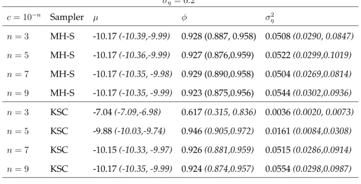
The estimated posterior medians and 95% credible intervals of the model pa-rameters for the two simulated data sets using the MH-S and KSC samplers are presented in Table 2. The MH-S sampler clearly provides estimates which are robust to the choice ofcover the range of values considered with both data sets. In contrast, the results using the KSC sampler depend on the value ofcwith both data sets. The larger values ofc (c = 10−3 andc = 10−5) provide extremely biased estimates for all summaries in both data sets. The method performs well with smaller values ofc

(c= 10−7andc= 10−9). This is not surprising since the mean ofy_t2isexp{µ+σ_η2/2}

which is4.6317×10−5 _{in this example and so is much smaller than the values}

(15)

σ_η = 0.2 c= 10−n _Sampler _µ _φ _σ2 η n= 3 MH-S -10.17(-10.39,-9.99) 0.928 (0.887, 0.958) 0.0508(0.0290, 0.0847) n= 5 MH-S -10.17(-10.36,-9.99) 0.927 (0.876,0.959) 0.0522(0.0299,0.1019) n= 7 MH-S -10.17(-10.35, -9.98) 0.929 (0.890,0.958) 0.0504(0.0269,0.0814) n= 9 MH-S -10.17(-10.35, -9.99) 0.923 (0.875,0.956) 0.0544(0.0302,0.0936) n= 3 KSC -7.04(-7.09,-6.98) 0.617(0.315, 0.836) 0.0036(0.0020, 0.0073) n= 5 KSC -9.88(-10.03,-9.74) 0.946(0.905,0.972) 0.0161(0.0084,0.0308) n= 7 KSC -10.15(-10.33, -9.97) 0.926(0.881,0.959) 0.0515(0.0286,0.0914) n= 9 KSC -10.17(-10.35, -9.99) 0.924(0.874,0.957) 0.0554(0.0298,0.0987) ση = 0.6 c= 10−n _Sampler _µ _φ _σ2 η n= 3 MH-S -10.17(-11.42,-8.89) 0.979(0.967, 0.990) 0.2010(0.1501, 0.2659) n= 5 MH-S -10.19(-11.46,-8.96) 0.980(0.967,0.990) 0.2004(0.1495,0.2721) n= 7 MH-S -10.19(-11.43, -8.86) 0.980(0.968,0.991) 0.1949(0.1509,0.2621) n= 9 MH-S -10.18(-11.37, -8.89) 0.979(0.967,0.990) 0.2027(0.1560,0.2051) n= 3 KSC -6.80(-7.04,-6.57) 0.978(0.958, 0.991) 0.0074(0.0043, 0.0120) n= 5 KSC -9.55(-10.49,-8.60) 0.983(0.972,0.992) 0.0803(0.0606,0.1063) n= 7 KSC -10.15(-11.36, -9.00) 0.980(0.968,0.990) 0.1870(0.1411,0.2462) n= 9 KSC -10.18(-11.37, -8.93) 0.979(0.966,0.990) 0.2069(0.1560,0.2763) Table 2: Posterior medians and 95%credible intervals of the model parameters with data simulated using different values ofc.

(16)

difference in the scales, an appropriate value would bec = 4.6317×10−8 which is contained in the range of vales forcfor which the KSC method performs well.

MH-S KSC 0 500 1000 1500 −12 −11 −10 −9 −8 −7 time h t 0 500 1000 1500 −12 −11 −10 −9 −8 −7 time h t

Figure 1: Posterior mean ofhtusing the MH-S and KSC methods and different values of c. The colour key for the line plots is: simulated (red),c= 10−3 _(blue),_c_{= 10}−5_(green),

c= 10−7_{(light blue).}

The KSC method should provide unbiased estimates of all parameters and so the biases in the posterior summaries forc= 10−3andc= 10−5are surprising. The plots in Figure 1 show the posterior means ofhtfor different samplers. Clearly, the

posterior mean ofht for the KSC sampler withc = 10−3 is larger than the correct

posterior values. This is directly due to the choice ofcwhich concentrates the poste-rior forhton larger values and so biases the results forµ. The importance sampler

should correct for differences but, in this case, the importance sampling distribu-tion places negligible mass on the correct values and so leads to biased posterior summaries. To confirm that this is the cause, we ran a Metropolis-Hastings chain without standardisation (i.e.where (6) is replaced bylog(y_t2+c) =ht+ logνt2))

(17)

(MH-c= 10−n _µ _φ _σ2 η n= 3 -7.64(-7,72, -7.58) 0.493(0.292, 0.665) 0.0033(0.0025, 0.0058) n= 5 -6.87(-6.85, -2.84) 0.949(0.398,0.967) 0.0057(0.0035,0.061) n= 7 -10.17(-10.35, -9.99) 0.925(0.876,0.957) 0.0539(0.0297,0.0960) n= 9 -10.17(-10.35, -9.98) 0.929(0.888,0.961) 0.0499(0.0274,0.0857)

Table 3: Posterior medians and 95%credible intervals of the model parameters with data simulated withση = 0.2and using the MH-NS sampler with different values ofc.

NS). Table 3 shows that this sampler also leads to biased estimates for smallc. This is an independence Metropolis-Hastings sampler which has a proposal supporting values far from the correct values of ht whenc = 10−3 and so the sampler never

moves to the correct values ofht.

The effective sample sizes for the two simulated data set using the MH-S and KSC samplers are presented in Table 4. These show that the MH-S sampler perform well for all values ofcdespite the length of the time series (T = 1500). The sampler has a large number of acceptedhmoves, good effective sample sizes forh100andµ,

and acceptable effective sample sizes for the other model parameters. The effective sample sizes with the KSC sampler are consistently larger for values ofcwhich give unbiased estimates of the posterior summaries (c= 10−7_and_c_{= 10}−9_{) .}

Overall, these results show that the MH-S method is robust to the choice of c

and can provide effective inference for relatively long time series (T = 1500) with realistic values of theφandση.

(18)

σ_η = 0.2 c= 10−n _Sampler _h 100 µ φ ση2 hmoves (%) n= 3 MH-S 1577.9 2952.9 143.9 76.2 40.5 n= 5 MH-S 1068.5 2230.3 96.8 58.9 27.2 n= 7 MH-S 1496.9 2625.1 76.6 76.6 41.2 n= 9 MH-S 1327.2 2050.1 67.5 67.5 29.0 n= 3 KSC 1672.1 181.4 36.0 109.5 n= 5 KSC 3055.6 3371.0 203.8 108.1 n= 7 KSC 3336.9 3430.8 210.0 138.5 n= 9 KSC 2590.7 3323.6 207.9 126.4 σ_η = 0.6 c= 10−n _Sampler _h 100 µ φ σ2η hmoves (%) n = 3 MH-S 693.1 3542.4 687.4 172.3 28.0 n = 5 MH-S 720.9 4092.8 465.6 126.3 25.5 n = 7 MH-S 860.9 3740.2 753.0 217.2 27.4 n = 9 MH-S 712.4 4209.0 950.0 238.1 25.3 n = 3 KSC 3392.3 3520.5 446.9 202.4 n = 5 KSC 2839.1 4135.3 1438.1 523.5 n = 7 KSC 2715.0 4103.0 1183.8 583.1 n = 9 KSC 3261.3 4016.6 1169.9 529.6

Table 4: Effective sample size for all model parameters with data simulated using differ-ent values ofc.

4.2 Eurostoxx Index

The returns of the Eurostoxx index from 2 January 2007 to 23 April 2013 were calcu-lated using the closing values and are shown in Figure 2. There are 1585 log returns

(19)

2007 2009 2011 2013 −0.05

0 0.05

daily log returns

Figure 2: Daily log returns of the Eurostoxx index from January 2007 to April 2013.

in the time series with 3 cases of zero log returns (on 6 January 2010, 3 March 2010 and 16 July 2012). The MH-S and KSC methods were run for different values ofc. An initial 20 000 iterations were used as a burn in period followed by a further 20 000 iterations which were thinned to 1 in 5 to sample the parameters.

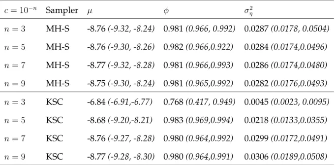
The estimated posterior median and 95% credible interval for this data set using the MH-S and KSC samplers are presented in Table 5. Again, these results show that the MH-S sampler provides good estimates of the posterior summaries for all value ofcwhereas the KSC sampler does not provide good summaries forc= 10−3. Again, this emphasises that the KSC sampler relies on a value ofcwhich is consistent with the scale of the data whereas the MH-S sampler works well regardless of the scale of the data.

Table 6 shows the ESS for both the MH-S and KSC samplers. The results are consistent with the simulated examples with the KSC sampler having a larger ESS than the MH-S but the MH-S providing a suitable ESS for effective inference.

(20)

c= 10−n _Sampler _µ _φ _σ2 η n= 3 MH-S -8.76(-9.32, -8.24) 0.981(0.966, 0.992) 0.0287(0.0178, 0.0504) n= 5 MH-S -8.76(-9.30, -8.26) 0.982(0.966,0.922) 0.0284(0.0174,0.0496) n= 7 MH-S -8.77(-9.32, -8.28) 0.981(0.966,0.993) 0.0286(0.0174,0.0480) n= 9 MH-S -8.75(-9.30, -8.24) 0.981(0.965,0.992) 0.0282(0.0176,0.0493) n= 3 KSC -6.84(-6.91,-6.77) 0.768(0.417, 0.949) 0.0045(0.0023, 0.0095) n= 5 KSC -8.68(-9.20,-8.21) 0.983(0.969,0.994) 0.0218(0.0133,0.0355) n= 7 KSC -8.76(-9.27, -8.28) 0.980(0.964,0.992) 0.0299(0.0172,0.0491) n= 9 KSC -8.77(-9.28, -8.30) 0.980(0.964,0.991) 0.0306(0.0189,0.0508) Table 5: Posterior medians and 95%credible intervals of the model parameters with the Eurostoxx data and using different values ofc.

c= 10−n _Sampler _h 100 µ φ ση2 hmoves (%) n= 3 MH-S 1709.4 3863.5 320.9 118.1 45.2 n= 5 MH-S 1772.0 3793.5 202.1 102.4 42.5 n= 7 MH-S 1771.6 3398.6 217.7 95.4 43.2 n= 9 MH-S 1253.8 3816.7 122.1 56.2 37.0 n= 3 KSC 3572.2 409.4 44.0 83.9 n= 5 KSC 3452.8 4001.1 572.1 217.7 n= 7 KSC 2823.0 3805.2 456.9 213.2 n= 9 KSC 3176.6 2960.0 347.0 157.5

Table 6: Effective sample size for all model parameters with the Eurostoxx data and using different values ofc.

(21)

The posterior medians ofhtis shown in Figure 3. The results from using a simpler 2007 2009 2011 2013 h t -11 -10 -9 -8 -7 -6

Figure 3: Posterior median ofhtfor the Eurostoxx data using the approximate variance to standardise the data.

standandardisation method are similar to the results shown in Figure 4 where the MH-S method was used.

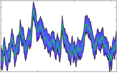
The posterior medians of ht(with the 95% credible interval) are shown in

Fig-ure 4. The volatility shows substantial persisetence and time-variation with higher values during the financial crisis.

4.3 Vector autoregression

The use of stochastic volatility in multivariate time series models has become in-creasingly common. As an example, we consider the following Bayesian VAR model with stochastic volatility which was introduced in Clark (2012) building on steady-state priors (Villani, 2009). Letytbe a(p×1)-dimensional vector of economics

(22)

2007 2009 2011 2013 h t -11 -10 -9 -8 -7 -6

Figure 4: Posterior median and 95% credible interval ofhtfor the Eurostoxx data using the MH-S withc= 10−3_.

measured at timet. The data modelled as

Π(L)(yt−Ψxt) =ǫt

whereΨis a(p×q)-dimensional vector of coefficients,Π(L) =Ip−Ψ1L−Ψ2L2. . .ΨkLk

is a lag polynomial andνtare independent errors. The vectorΨxtallows for a

deter-ministic trend within the model. The errorsǫtare modelled using a factor stochastic

volatility model. LetAbe a lower triangular matrix with 1’s on the diagonal then

ǫt=A−1Λ0t.5νt, νt∼N(0, Ip),

Λt=diag(eh1,t, eh2,t, . . . ehp,t),

hi,t =hi,t−1+ση,iηi,t, ηi,tiid∼ N(0,1) ∀i= 1,2, . . . , p.

Clark (2012) applies the model to output growth, unemployment rate, inflation and federal funds rate with long-term inflation expectations used as an exogeneous

(23)

variable and uses real-time data from 1961:Q1 to 2008:Q3. We consider the same data and time period but use the final revision values for all data.

Clark (2012) describes, in detail, the prior specification and the Gibbs sampling steps needed to fit the model and these are not repeated here. The full conditional distribution for each volatility process can be put in the form of a stochastic volatility model by noting that

AΠ(L)(yt−Ψxt)≡y˜t= Λ0t.5νt

and

log ˜y_i,t2 =hi,t+ logνi,t2 , ∀i= 1, . . . , p.

This allows the KSC method described in Section 2 to be used to updatehi,1, . . . , hi,T

from their full conditional distribution for eachi= 1, . . . , pin a Gibbs sampler. How-ever, Clark (2012) notes that “in preliminary investigations with BVAR models, es-timates based on the latter algorithm seemed to be unduly dependent on the priors and prone to yielding highly variable estimates of the volatility”. Therefore, we con-sider the MH-S algorithm described in Section 3 and show that this algorithm is able to successfully sample from the posterior distribution. The posterior distribution of the model was sampled using 3 different values of the mixture offset (c = 10−3_,

c= 10−6 _and_c _{= 10}−9_{) with the sampler from for a total of 50 000 iterations with a}

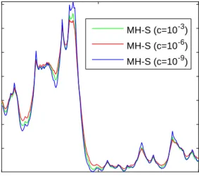
burn-in period of 10 000 iterations. The results were found to be very similar for all parameters and very similar to results from a Metropolis-Hastings algorithm which updates eachhi,tseparately without taking any transformations. For iilustration, the

posterior median ofeh1,t _{for the three values of}c_{are shown in Figure 5 and clearly}

(24)

1961 1985 2008 0.6 0.8 1 1.2 1.4 1.6 1.8 MH-S (c=10-3) MH-S (c=10-6) MH-S (c=10-9)

Figure 5: Posterior median ofeh1,t_{for Example 4.3 using different mixture offset values}

and the MH-S method.

5 Conclusion

When the SV model is expressed in linear state space form using a normal mixture model, the value of the offset parameterc used for the MCMC sampling can have an important effect on the posterior inferences. To overcome this lack of robustness to the choice ofc, we propose a Metropolis-Hastings sampler which uses a linear state space constructed using a standardised version of the error term. The volatili-ties are sampled jointly using a forward filtering backwards sampling algorithms in the same way as KSC. This approach provides inference about the volatility and the model parameters which is robust to the choice ofc The effective sample sizes for the volatility and the model parameters indicate that the method can provide accu-rate inference for realistic values of the model parameters on time series of realistic length.

(25)

conditional joint distribution for the volatilities and so no importance sampling re-weighting is needed to correct inference. The application to a vector autoregression with stochastic volatility in section 4.3 shows that sampling from the correct full conditional distribution can have important consequences for the ability of the Gibbs sampler to simulate from the correct posterior distribution.

References

Atchade, Y. and S. Rosenthal (2005). On adaptive Markov chain Monte Carlo algo-rithms. Bernoulli 11(5), 815–828.

Belmonte, M. A. G., G. Koop, and D. Korobilis (2013). Hierarchical shrinkage in time-varying parameter models. Journal of Forecasting 33, 80–94.

Bollerslev, T. (1986). Generalized autoregressive conditional heteroskedasticity. Jour-nal of Econometrics 31, 307–327.

Carter, C. K. and R. Kohn (1994). On Gibbs sampling for state space models.

Biometrika 81(3), 541–553.

Chib, S., F. Nardari, and N. Shephard (2002). Markov chain Monte Carlo methods for stochastic volatility models. Journal of Econometrics 108(2), 281–316.

Clark, T. E. (2012). Real-time density forecasts from Bayesian vector autoregressions with stochastic volatility. Journal of Business & Economic Statistics.

De Jong, P. and N. Shephard (1995). The simulation smoother for time series models.

Biometrika 82(2), 339–350.

(26)

Engle, R. F. (1982). Autoregressive Conditional Heteroscedasticity with Estimates of the Variance of United Kingdom Inflation. Econometrica 50(4), pp. 987–1007. Fr ¨uhwirth-Schnatter, S. (1994). Data augmentation and dynamic linear models.

Jour-nal of Time Series AJour-nalysis 15, 183–202.

Fuller, W. A. (2009). Introduction to statistical time series, Volume 428. John Wiley & Sons.

Harvey, A. C. and N. Shephard (1996). Estimation of an asymmetric stochastic volatility model for asset returns. Journal of Business & Economic Statistics 14(4), 429–434.

Jacquier, E., N. G. Polson, and P. E. Rossi (1994). Bayesian analysis of stochastic volatility models. Journal of Business & Economic Statistics 12, 371–389.

Jensen, M. J. and J. M. Maheu (2014). Estimating a semiparametric asymmetric stochastic volatility model with a Dirichlet process mixture. Journal of Economet-rics 178, 523–538.

Kastner, G. and S. Fr ¨uhwirth-Schnatter (2014). Ancillarity-sufficiency interweav-ing strategy (ASIS) for boostinterweav-ing MCMC estimation of stochastic volatility models.

Computational Statistics & Data Analysis 76, 408–423.

Kim, S., N. Shephard, and S. Chib (1998). Stochastic Volatility: Likelihood Inference and Comparison with ARCH Models. The Review of Economic Studies 65(3), pp. 361–393.

Omori, Y. and T. Watanabe (2008). Block sampler and posterior mode estimation for asymmetric stochastic volatility models. Computational Statistics & Data Anal-ysis 52(6), 2892–2910.

(27)

Sokal, A. (1997). Monte Carlo methods in statistical mechanics: foundations and new algorithms. InFunctional integration, pp. 131–192. Springer.

Villani, M. (2009). Steady-state priors for vector autoregressions. Journal of Applied Econometrics 24, 630–650.

A

Derivation of the Metropolis-Hastings acceptance

ratio for sampling

h

The Metropolis-Hastings acceptance ratio is

a=min 1,pq(h ′ , θ, s|y) pq(h, θ, s|y) q(h|h′, θ, y, s) q(h′ |h, θ, y, s) ! , =min 1,p(y|h ′ , θ)p(h′|θ)g(s|h′, θ, y) p(y|h, θ)p(h|θ)g(s|h, θ, y) q(h|h′, θ, y, s) q(h′_|_{h, θ, y, s}₎ ! . Using q(h|h′, θ, y, s) = p˜(y|h, θ, s)p(h|θ) ˜ p(y|s, θ) , and g(s|h′, θ, y) = p˜(y|h ′_{, θ, s}_)˜_p₍_s₎ ˜ p(y|h′_{, θ}₎ , implies that a=min  1, p(y|h′_{, θ}₎_p₍_h′_|_θ₎ p(y|h, θ)p(h|θ) ˜ p(y|h′_,θ,s_)˜_p₍_s₎ ˜ p(y|h′_,θ₎ ˜ p(y|h,θ,s)˜p(s) ˜ p(y|h,θ) ˜ p(h,θ,s)p(h|θ) ˜ p(y|s,θ) ˜ p(y|h′_,θ,s₎_p₍_h′_|_θ₎ ˜ p(y|s,θ)  .

Finally, cancelling out the terms, gives

a=min  1, p(y|h,θ) ˜ p(y|h′_,θ₎ p(y|h,θ) ˜ p(y|h,θ)  .