A Study of a Formal Model
For View Selection for Aggregate Queries
Zohreh ASGHARZADEH TALEBI1
, Rada CHIRKOVA2
, and Yahya FATHI1
1
Operations Research Program, NC State University, Raleigh, NC 27695,
{zasghar,fathi? ? ?}@ncsu.edu 2
Computer Science Department, NC State University, Raleigh, NC 27695,
Abstract. We present a formal study of the following view-selection problem: Given a set of queries
and a database, return definitions of views that, when materialized in the database, would reduce
the evaluation costs of the queries. Optimizing the layout of stored data using view selection has a
direct impact on the performance of database systems. At the same time, the optimization problem is
intractable, even under natural restrictions on the types of queries of interest. We introduce an
integer-programming model to obtain optimal solutions for the view-selection problem for aggregate queries on
data warehouses. We show that this model can be used to solve realistic-size instances of the problem.
We also report the results of the post-optimality analysis that we performed to determine the impact of
changing certain input characteristics on the optimal solution, and compare our approach to a leading
heuristic procedure [20]. A shorter version of some results of this paper has been published as [25].
1
Introduction
As relational databases and data warehouses keep growing in size, evaluating many
com-mon queries — such as aggregate queries — by database-management systems (DBMS)
may require significant transformations of large volumes of stored data. As a result, the
re-quirement of good overall performance of frequent and important user queries necessitates
? ? ? This author’s work is partially supported by the National Science Foundation under Grant No. 0321635.
optimal DBMS choices in choosing and executing query plans. A significant aspect of query
performance is the choice of auxiliary data used in query answering, such as which indexes
are used in a query plan to access a given stored relation. In modern commercial database
systems, another common type of auxiliary data is materialized views— relations that were
computed by answering certain queries on the (original) stored data in the database and that
can be used to provide, without time-consuming runtime transformations, “precompiled”
in-formation that is relevant to the user query. We give an example of using materialized views
to answer select-project-join queries with aggregation in a star-schema [22] data warehouse.
Example 1. Consider a star-schema data warehouse with three stored relations:Sales(CID,
DateID,QtySold,Discount), Customer(CID,CustName,Address,City,State), and
Time(DateID, Day,Week,Month,Year); here,Sales is the fact table.
Let the query workload have two queries, Q1 and Q2. Q1 asks for the total quantity of
products sold per customer in the last quarter of the year 2005.Q2asks for the total product
quantity sold per year for all years after 2000 to customers in North Carolina.
Q1: SELECT c.CID, SUM(QtySold) Q2: SELECT t.Year, SUM(QtySold) FROM Sales s, Time t, Customer c FROM Sales s, Time t, Customer c
WHERE s.DateID = t.DateID AND s.CID = c.CID WHERE s.DateID = t.DateID AND s.CID = c.CID AND Year = 2005 AND Month >= 9 AND Month <= 12 AND Year > 2000 AND State = ‘NC’
GROUP BY c.CID; GROUP BY t.Year;
We can use techniques from [20] to show that the following view V can be used to give
exact answers to each of Q1 and Q2.
That is, suppose the view V is materialized in the data warehouse, which means that
the answer to the query V on the database is precomputed and stored as a new relation
V3
alongside Sales, Customer, and Time. Then the answer to each of Q1 and Q2 can be
computed by accessing just the data in the relationV. For instance, Q1 can be evaluated as
Q1: SELECT CID, SUM(SumQS) FROM V WHERE Year = 2005 AND Month >= 9 AND Month <= 12 GROUP BY CID;
Note that evaluating the queryQ1 using the viewVis likely to be more efficient than
evaluat-ing Q1using its original definition, as usingV allows the DBMS to avoid taking an expensive
join ofSales,Customer, andTimeand also may save some time in grouping and aggregation.
We consider the followingview-selection problem:Given a set of queries, a database, and a
set of constraints (e.g., a storage limit on the amount of disk space that can be used to store
materialized views), return definitions of views that, when materialized in the database,
would satisfy the constraints and reduce the evaluation costs of the queries. As design of
materialized views is an important component of query processing in data warehouses [7, 20,
31, 35, 38] and of automated query-performance tuning [21, 28, 30], the problems of selecting
views and of answering queries using views have been studied thoroughly in the literature.
Generally, spending more time on designing views tends to pay off, as greater
improve-ment can thereby be achieved in the query performance using the resulting stored derived
data. As the number of beneficial views or indexes tends to be prohibitive even for simple
query workloads [3, 12, 20], it is not practical to use exhaustive enumeration to obtain derived
data that would globally minimizequery costs. Several approaches (see, e.g., [3, 18, 20, 31])
3
have been proposed to efficiently design good-quality sets of derived data for SQL queries.
We continue the work of [18, 20] of studying view-selection algorithms that are competitive,
that is, provide optimality guarantees on their outputs without necessarily exploring the
entire search space of views. We present a formal model of view selection for queries on
star-schema data warehouses and explore competitive techniques for designing and using views
in this context. Our techniques and results are applicable to a practically important class of
range-aggregate queries on star-schema data warehouses.
Our contributions are as follows:
(1) we model view selection as an integer-programming (IP) problem and give references to
similar IP structures in the literature (Section 3),
(2) we use standard IP-solver software (CPLEX [29] with an AMPL interface [15]) to solve
optimally realistic-size instances of the problem on the popular TPC-H benchmark [36]
and on real data in the Sloan Digital Sky Survey (SDSS) dataset [34] (Sections 4–6),
(3) we study the limits of our approach for two versions of the view-selection problem,
de-termined by whether the table for the view resulting from joining all the base relations
(we call this view raw-data view) is part of the solution (Sections 3 and 5), and
(4) we experimentally compare our method with a leading heuristic approach in the field [20],
and theoretically analyze the worst-case performance of that approach (Section 6).
In our experiments we solved hundreds of problem instances, both on TPC-H data [36]
and on the SDSS dataset [34]. The problem instances used both randomly generated query
After outlining related work, in Section 2 we provide the background and formal
defini-tions. Section 3 introduces our IP model of the view-selection problem. Section 4 describes
our framework for analysis and experimentation. We report our experimental results and
theoretical analysis in Sections 5 and 6, and conclude in Section 7.
Related Work
Designing and using derived data to improve query performance has long been studied in
data-intensive systems. A wealth of theoretical results (see [19] for a survey) and some
practi-cal solutions [4, 10, 11] have been accumulated on using views and indexes in query answering.
Answering aggregate queries using views was considered in relation to data warehouses and
data cubes [2, 9, 16, 37]; results on answering each query using a single view were presented
in [17, 33]. Recent work [1, 13] considered rewriting aggregate queries using multiple views.
Considerable work has been done on efficiently selecting views and indexes for general
SQL queries [3] and in particular for aggregate queries (e.g., [1, 18, 20, 31]). [38] proposed
algorithms, including an IP approach, for selecting materialized views to minimize the sum
cost of processing the given queries and of maintaining all the views. [3, 4] introduced an
end-to-end approach and a system architecture for designing and using materialized views and
indexes to answer queries. In this paper we study the problem of selecting views for aggregate
queries on star-schema data warehouses. The setting and assumptions we use generalize those
in [18, 20] (in contrast to those in [38]) — that is, we seek to minimize the total execution
costs of q given set of queries under a storage-limit constraint. At the same time, the novelty
sizes, for two versions of the view-selection problem. In the first version, we assume similarly
to [20] that the raw-data view is always part of the solution set of materialized views. We
lift this restriction in the second version of view selection; the resulting problem arises in
practice in settings where it is too expensive to maintain efficiently the result of joining
all base tables, including data-integration settings where certain views are materialized in
the mediator to improve query-processing efficiency [19]. In our current work we are using
lower-bound relaxation in developing competitive heuristics for problem instances that are
too large to be solved optimally, for both versions of the view-selection problem.
2
Preliminaries and Problem Specification
The setting we use is similar to that in [18, 20]. We consider relational select-project-join
queries with equality-based joins and with aggregation functions sum, count, max, or min.
Our approach is applicable to queries with inequality comparisons of attributes to constant
values, including the important class of range-aggregate queries. We study parameterized
queries: The parameterized version of a query has placeholders instead of all the constants.
In this paper we focus on the special case of star-schema queries: We assume that the
database schema is a star schema [22], with a fact table and dimension tables. Further, in
each star-schema query, each join is a natural join of the fact table with a dimension table.
Our cost model is as follows. We consider the costs of answering queries using unindexed
materialized views, such that each query can be evaluated using just one view relation and no
each query is proportional to thesizeof the view chosen for the evaluation. We use two metrics
for view sizes: (1) the number of rows in the view relations (this is a common assumption
in the literature on view selection), and (2) the number of bytes in the view relations. In
Section 5 we will see that these metrics give us different experimental results. Finally, given
a query workloadQ and a set of viewsV that have been precomputed on a database D, the
total cost of evaluating Qusing V is the sum of the costs of evaluating all the queries in Q, such that each query is evaluated using a view in V. The sum can be weighted to reflect the relative frequency or importance of individual queries. We consider two settings: In the first
setting, similarly to [20] we assume that a view resulting from joining all the base relations
in the star schema — we call it the raw-data view — is always part of the available setV of materialized views. We lift this assumption in the other setting considered in this paper.
We consider the following view-selection problem: Our goal is to minimize the evaluation
costs of a given workload of parameterized aggregate queries defined on a star schema, by
selecting and precomputing views that can be used in answering the queries. (We consider
only equivalent query rewritings, i.e., we require that exact answers to all the queries in Q
can be computed using V.) We consider this minimization problem under a storage-space limit, which is an upper bound on the amount of disk space that can be allocated for the
views. Thus, ourproblem inputsare of the form I = (D,Q, b), whereD is a database, Qis a workload of parameterized queries, and b is the (positive integer) value of the storage limit.
For any parameterized query in the given workload, our goal is to design views that can
views without comparisons with constants. We use the following definitions of solutions and
of the optimal viewset problem (OV P):
Definition 1. For a problem input I = (D,Q, b), a set of viewsV is anadmissible viewset
if (1) each query in Q can be rewritten using V, and (2) V satisfies the storage limit b.
Definition 2. For a problem input I = (D,Q, b), an optimal viewset is a set of views V
defined on D, such that (1) V is an admissible viewset for I, and (2) V minimizes the cost of evaluating Q on the database DV, among all admissible viewsets for I. Here, DV is the
database that results from adding to D the relations for all the views in V computed on D.
Definition 3. (Problem OV P) For a given problem input I = (D,Q, b), find an optimal viewset. A solution for a given instance of OV P consists of a set of materialized views V
(which includes the raw-data view onDand all additional views that we choose to materialize) and an association between each element of Q and its corresponding element of V.
As we mentioned earlier in this section, we also consider a variationOV P0
of the
optimal-viewset problem: Unlike OV P, in OV P0
we do not require that the raw-data view be
mate-rialized as part of the solution. In Section 5 we present an experimental comparison of two
versions of our proposed approach, one for OV P and the other for OV P0
.
3
The Formal Model
In this section we propose an integer programming (IP) model for the optimal-viewset
prob-lems OV P and OV P0
, and discuss methodologies for solving this IP model. We use the
ai : Size of the viewi, for all i ∈ IV, where IV is the index set for all possible views;
b: storage limit;
cij: evaluation cost of answering queryj by using view i, for all i ∈ IV and j ∈ Q.
We let cij = +∞ if view i cannot be used to answer query j. We further define the
following decision variables for the IP model.
xi =
1 if view i is materialized
0 otherwise
for all i ∈ IV
and
yij =
1 if we use view i to answer query j
0 otherwise
for all i ∈ IV and j ∈ Q
The optimal-viewset problemOV P can now be stated as the following IP modelOV IP.
Minimize P
i ∈ IV P
j ∈ Qcijyij (OV IP)
subject to P
i ∈ IV aixi ≤b (1)
P
i ∈ IV yij= 1 for all j (2)
yij≤xi for all i, j such that cij 6= +∞ (3)
x1 = 1 (4)
xi, yij ∈ {0,1} for all i, j
Constraint (1) limits the size of the views to be no more than the storage space b.
Constraint (2) states that each query is answered by exactly one view in the set of views.
materialized. Constraint (4) states that the raw-data view is always materialized, and the
remaining constraints are simply the binary requirements forxi andyij. Note that the binary
requirement for yij can be replaced by a simple non-negativity restriction without affecting
the corresponding optimal solution for this model. This relaxation, however, has a significant
impact on reducing the overall computational effort required to solve this IP model.
We can also modify this model into an IP model for the problem OV P0
by removing
constraint (4). This is equivalent to stating that the raw-data view is not required to be
materialized. We refer to this modified model, i.e.,OV IP without constraint (4), as OV IP0
.
The structure of this IP model is similar to those for the uncapacitated facility location
problem (UFL) and the k-median problem. These two problems are well studied in the
literature, and relatively large instances of the corresponding IP models can be solved within
reasonable time. Several heuristic approaches for solving these problems have also been
reported. See [14] and [24] for the facility location problem and [26] for thek-median problem.
We can also employ the linear programming (LP) or Lagrangean relaxation of this IP
model to develop lower bounds for the optimum solutions. [32] observed that the LP
re-laxation for the facility location problem can provide strong lower bounds for it, and [27]
showed that the Lagrangean relaxation can provide even better lower bounds. Due to the
similarity of the structure of OV IP (OV IP0
) with these models we expect that similarly
strong lower bounds can be obtained for OV IP (OV IP0
). As these bounds are typically
obtained with modest computational effort, we could use them to devise exact algorithms
for each instance to evaluate the solution obtained via a heuristic procedure, hence providing
an upper bound on the performance ratio of the algorithm in that instance.
4
Our Framework
We consider view selection for star-schema queries. To design aggregate views for star-schema
queries, we use a data structure,view lattice, that was introduced in [20]. A view lattice is a
representation of the search space of views for a problem input, where nodes represent views
and directed edges between the nodes denote which view can be evaluated using another
view. For any view we choose to materialize, if the view is usable in evaluating an input
query, then the answer to the view is the only relation needed in the evaluation. That is,
our view-selection procedures determinejoinlessrewritings of queries (see [1, 13] for work on
rewritings computed via joins of aggregate views with other relations).
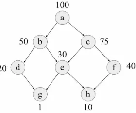
Fig. 1.Lattice example with space
costs [20].
To define an instance of the problem and to construct
input data for our IP formalism, we first select a query
work-load, that is, frequent and important queries whose
evalu-ation costs we want to reduce by materializing views. We
then use the approach of [20] to construct a view lattice, by
associating each workload query with a node in the lattice.
More specifically, we construct from the query workload a set of grouping and aggregated
attributes of interest — these are all the attributes mentioned in the queries, except the
as described in [20]. For instance, suppose queries Q1 and Q2 in Example 1 comprise our
workload queries. We use attributes mentioned in Q1 and Q2 to construct the grouping and
aggregated attributes of interest — CID, Year, Month, State and QtySold, respectively.
Once we have constructed a view lattice, we calculate the sizes of the answers to all
the views in the lattice. We can estimate the sizes by using methods mentioned in [20], for
instance sampling. Finally, to complete the input data, we specify a storage limit.
To illustrate, we present an example adopted from [20]. Figure 1 shows the view lattice
for this example that consists of the raw-data view (node a) and of views {b, c, d, e, f, g, h}. The space requirement is given next to each node, and the edges represent the relationship
between views as discussed above. We assume that the query workload consists of all nodes
in the lattice, and the problem is to determine a set of at most three additional views
to materialize (in addition to the raw-data view a) that would minimize the total cost of
answering the workload queries. Note that to be consistent with the example given in [20]
we restrict the number of views, rather than their corresponding storage space requirement.
The IP model (OV IP1) for this example can be written as follows:
Minimize P8
i=1 P8
j=1cijyij (OV IP1)
subject to P8
i=1xi ≤4 P8
i=1yij = 1 for all j = 1 to 8
yij≤xi for all i, j such that cij 6= +∞
x1 = 1
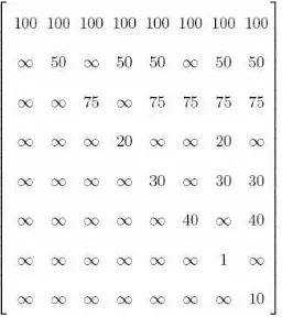
Fig. 2.Cost matrix forOV IP1.
The matrix of objective-function coefficients cij for
the model OV IP1 is shown in Figure 2, where nodes
a, b, c, d, e, f, g,and hcorrespond to the rows (and columns)
1 through 8, respectively. The model OV IP1 has 8 binary
variables and 64 continuous variables. We solved this
prob-lem using the IP solver CPLEX [29] with an AMPL
inter-face [15] and obtained the optimal solution x1 =x2 =x4 =
x6 = 1 (corresponding to nodes a, b, d, f in the lattice), y11 =y22=y13 =y44 =y25 =y66=
y47 = y68 = 1, with all other variables equal to zero. The total cost associated with this
solution is 420. Incidentally, this solution is identical to the solution in [20].
To represent the lattice associated with a large data set (for a realistic instance of view
selection), we use a table format. Each row in the table corresponds to a lattice node; the
two entries in each row represent the view ID and the view sizefor that node, respectively.
Thus, the table has two columns and as many rows as the number of lattice nodes.
In each row (i.e., node of the lattice) the view size is represented in units that we choose
for our analysis (e.g., number of rows in the view, number of bytes of stored data in the
view, etc.), and the view ID is a binary vector of size K. The ith element in the vector is
the ith grouping attribute, andK is the total number of grouping attributes. For each view,
an entry of 1 in the ith position of its view ID implies that the corresponding attribute is
used to group the associated rows in the database (to form this view). In other words, a 1
to answer a query that requires the ith attribute, and a 0 entry in the ith position implies
otherwise. We give SQL examples in Section 5; see Appendix B in [6] for a full description
of one instance of view selection on TPC-H data [36] and its solution.
Thus, dependencies among nodes can be derived from their view IDs. A query e can be
computed from a view f (i.e., f is an ancestor of e in the lattice) if the set of positions
with entry 1 in the view ID for e is a subset of the respective set in the view ID for f (e.g.,
f = {1,1,0,0,1} is an ancestor for e = {0,1,0,0,1}, but it is not an ancestor for e0
=
{0,1,0,1,0}). Note that the number of nodes in the lattice is 2K and increases exponentially
as the number of attributes K increases. For this reason, in order to keep the size of the IP
model as small as possible, in each instance we only maintain those nodes of the lattice that
are potential ancestors of at least one query in our query workload for that instance.
The evaluation cost of a query e using a viewf is the storage cost of the view f if e can
be answered by f, and is ∞ otherwise. Following the above criteria, the cost matrix for a query workload can be easily computed and transformed to the input of the IP model.
5
Experimental Evaluation of our Approach
We have conducted extensive experiments to evaluate the IP models and framework presented
in Sections 3 and 4. (For each experiment type, we have solved many more instances of the
problem than are described in this and next sections. For a report on all the instances,
please see [5, 6].) All experiments were run on a machine with a 3GHz Intel P4 processor,
Region Nation2 Nation1 Orders Customer PartSupp Supplier Part Lineitem 396 2,103 2,103 482,877,440 244,883,456 5,830,541 14,188,544 1,193,906 2,147,483,647 Size (bytes) Name TPC-H Tables
Fig. 3.Sizes of TPC-H tables.
In this section we outline an experimental evaluation of
our approach; in Section 6, we compare our approach with the
state-of-the-art algorithm of [20]. We did all the experiments
on two datasets: (1) on a TPC-H database benchmark [36],
and (2) on real data, using a modified Sloan Digital Sky
Sur-vey (SDSS) dataset [34]. Figure 3 shows the sizes of the stored tables for the TPC-H dataset.
Size estimates for the lattice were obtained by running the queries for all views on the TPC-H
stored data with scale factor of 0.1 and by extrapolating the answer sizes to the sizes of the
data (scale factor of 1) used in the experiments. For the SDSS dataset, whose sizes of the
stored tables are shown in Figure 4, the view sizes were measured on the original database.
The observations we made in our experiments were consistent across the two datasets;
there-fore, in reporting our results we will use examples just from the TPC-H dataset.
Neighbors Field Segment Plate PhotoObj SpecObjAll 1,321 919 621 69,035 38,206,539 200,851,705 Size (bytes) Name SDSS Tables
Fig. 4.Sizes of SDSS tables.
The goal of the experiments that we report in this section
was to obtain optimal solutions and lower bounds on instances
of OV IP and OV IP0
of realistic sizes. The experimental
re-sults show the following:
– relatively large instances of the view-selection problem, including instances of realistic
sizes, can be solved optimally within reasonable execution time;
– the LP relaxation provides a strong lower bound for the corresponding optimal value;
– regardless of whether we use the number of rows or the number of bytes for measuring
corresponding optimal solution of the view-selection problem, and in many instances the
respective optimal solutions are not identical;
– in many instances the optimal solution for OV IP0
is different from that for the
corre-spondingOV IP problem, and the value of the objective function is significantly smaller.
The experimental results that we present in Section 6 further demonstrate that the overall
computational effort required to solve an instance of the problem using our proposed IP
model (i.e., the time required to find an optimal solution for a problem instance) is
substan-tially smaller than that required to solve the same instance using the heuristic procedure
proposed in [20] (i.e., to find a potentially sub-optimal solution for the same instance).
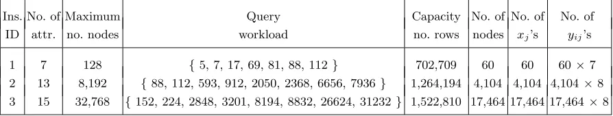
Ins. No. of Maximum Query Capacity No. of No. of No. of ID attr. no. nodes workload no. rows nodes xj’s yij’s
1 7 128 {5, 7, 17, 69, 81, 88, 112 } 702,709 60 60 60×7 2 13 8,192 {88, 112, 593, 912, 2050, 2368, 6656, 7936} 1,264,194 4,104 4,104 4,104×8 3 15 32,768 {152, 224, 2848, 3201, 8194, 8832, 26624, 31232} 1,522,810 17,464 17,464 17,464×8
Table 1.Description of three problem instances in the experiments.
5.1 Solving the Problem Instances
For the experiments that we report here we used four TPC-H datasets — raw-data views with
7, 13, 15, and 17 attributes, respectively. (To obtain some raw-data views for the experiments,
we used joins of TPC-H tables.) The numbers of nodes in the view lattices for these datasets
are 128, 8192, 32768, and 131072, respectively. For each raw-data view we constructed the
IP model OV IP for several instances of the problem, each instance with a different query
workload and storage limitb. For each instance, given the view lattice, query workload, and
solved each instance using the software package CPLEX/AMPL, and in each instance on
datasets with 7, 13, and 15 attributes we were able to find an optimal solution. In Table 1
we give detailed characteristics of three different problem instances in our experiments. Each
row of this table corresponds to one instance and gives the view lattice (raw-data view)
and query workload corresponding to that instance. The maximum number of nodes in each
instance is 2K, where K is the number of attributes in the view lattice. Note that in our IP
model we only include those nodes that could be used as potential ancestors for one or more
queries in the query workload for that instance. Thus, the number of nodes we included in
the IP model is in fact smaller than 2K, as stated in the table. For each instance we also
give the number of variables in the corresponding IP model.
We now explain how to read the IDs of queries and views in Table 1 and in the other
tables in this and next sections. Recall that by construction of the view lattice, there is a
one-to-one relationship between aggregate queries/views on the raw-data view and nodes in
the view lattice. We order the grouping attributes of the raw-data view from left to right
and index each node in the lattice using the decimal representation of the list of 1/0 bits
that is constructed as described in Section 4. As the root node of the view lattice always has
exactly the grouping attributes of the raw-data view, the decimal index of the root node is the
decimal encoding of a list that has only 1’s. To illustrate the assignment of indexes to queries
and views in Tables 1 and 2, we give the definition of view 55 and one possible definition of
query 55 (see instance 1 in Table 2) on the list of attributes Orderkey, Suppkey, Partkey,
View55: SELECT Suppkey, Partkey, Linestatus, Shipdate, Discount, SUM(Extendedprice) FROM Lineitem GROUP BY Suppkey, Partkey, Linestatus, Shipdate, Discount;
Query55: SELECT Suppkey, Partkey, Linestatus, SUM(Extendedprice) FROM Lineitem
WHERE Discount < 0.2 AND Shipdate = ‘2005-08-01’ GROUP BY Suppkey, Partkey, Linestatus;
Recall that each query is associated with a node that has as grouping attributes all
attributes mentioned in the GROUP BY and WHERE clauses of the query. Thus, the attributes
Discount and Shipdate ofView55 appear in theWHEREclause inQuery55. (The aggregated
attribute Extendedprice is not represented in the view lattice, similarly to [20].)
5.2 Execution Time
2 4 6 8 10 12 14 16
13 14 15 16 17 18 19 20 21 22 Optimal Cost LP lower bound
X105 X105 C o s t
Storage Limit, b
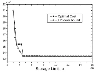
Fig. 5. Sensitivity analysis and LP
lower bound for the view-7 instance.
The execution time for CPLEX/AMPL to solve the three
instances in Table 1 was 0.12 seconds, 0.45 seconds,
and 3.89 seconds, respectively. The execution time is
ex-pected to grow at an exponential rate with the size of
the IP model; hence we do not expect it to be
practi-cal to solve much larger instances of this IP model using
CPLEX/AMPL. At the same time, the instances that we are able to solve are of realistic sizes
in practice, as exemplified in the three instances described in Table 1. This demonstrates
that we can use a standard IP solver to solve practical instances of our proposed IP model.
Aside from the number of attributes and queries, the size (and execution time) of the IP
model also depends on the number of lattice nodes that are actually included in the model,
number is usually larger if some workload queries are placed relatively low in the lattice.
Hence, the largest IP model in our experiments does not necessarily pertain to the lattice
with the largest number of attributes. In fact, the largest IP model that we were able to solve
optimally was for instance 3 in Table 1, which is on a 15-attribute lattice with 8 queries,
and its execution time was 3.89 seconds. The largest instance of OV P that we were able to
solve, however, pertains to a 17-attribute lattice with 15 randomly generated queries, and its
execution time was only 2.64 seconds, see [5]. The number of nodes included in the former
IP model is 17,464 (see Table 1), while in the latter is 13,755. Further, the largest IP model
does not necessarily pertain to the longest execution time, since the latter also depends on
the growth of the search tree in the context of the branch and bound algorithm. In fact, the
longest execution time in our experiments pertains to an instance with a 7-attribute view
lattice and 50 queries (instance 14 in Table 4); its execution time was 13 seconds.
In many instances, while solving the IP model we also observed that the runtime of
CPLEX/AMPL for solving the model is only slightly larger than its runtime for solving
the corresponding LP model. Intuitively, the lower bound obtained via the LP model is a
relatively strong lower bound, hence it leads to quick fathoming of most branches in the
corresponding branch-and-bound tree. In our experiments, every time that CPLEX/AMPL
was not able to solve the IP model within our stated time limit, it was also unable to solve
its LP model. We report on the quality of this lower bound in the next subsection.
Note that the heuristic approach of [20] (see Section 6) was much less effective, in terms
In our experiments we also studied whether the ancestor-descendant relationships
be-tween workload queries influence the runtime or outcome for our approach. In particular,
we studied problem instances with “single-path” query workloads, that is, with workloads
Q where for each query Q ∈ Q, each remaining query in Q is either a descendant or an ancestor of Q in the view lattice. It has been observed in [23] that workload queries with
such relationships are likely to occur in query sessions by a single user in data warehouses,
where the user performs roll-ups and drill-downs on the data of interest. In our study, we did
not observe significant differences in the runtime or outcome for our approach depending on
the type of relationships among workload queries. Rather, as mentioned earlier, we observed
that the placement of individual queries in the view lattice has a bigger influence on how
efficiently the problem instance can be solved by our approach.
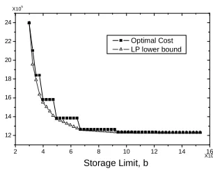
5.3 Post-Optimality Analysis
2 4 6 8 10 12 14 16
12 14 16 18 20 22 24 Optimal Cost LP lower bound
X105 X105 C o s t
Storage Limit, b
Fig. 6. Sensitivity analysis and LP
lower bound for the view-13 instance.
We have performed a post-optimality analysis to observe
the impact of changing the storage limit b on the
opti-mal value of the objective cost function. In realistic
view-selection scenarios, the total space available to store the
materialized views is usually smaller than the total size of
the relations for the input query workload; otherwise we
can precompute all the queries in advance and store them on disk, which would be a globally
optimal solution to the view-selection problem. At the same time, the storage limit has to
that the raw-data view must be materialized, as in OV IP0
). Hence, to explore the tradeoff
between the amount of available storage space and the resulting total query costs, in our
experiments we varied the value of storage space b between one and five times the size of
the raw-data view. Figures 5 and 6 show the results for two instances of Table 1, with 7 and
13 attributes respectively. In each instance and for each value of b we also solved the
corre-sponding LP problem to obtain the associated lower bound; the lower bounds are also shown
on the graphs. (The step curves in Figures 5 and 6 give the optimal cost value, whereas the
smooth curves show the lower bounds.) Intuitively, the optimal cost changes only when the
value of b increases sufficiently to allow for a different combination of materialized views to
be the optimal solution. Hence, as we increase the value of b, we observe a stepwise decrease
in the optimal cost only at those values ofbthat would allow sufficient capacity for a different
(better) collection of materialized views. Note that if the storage capacitybis so limited that
we can only store the raw-data view, then each query would be computed directly from that
view; the optimal query cost decreases monotonically as we increase the value of b. Finally,
we observe that the LP lower bound is very close to the optimal value of the IP problem
most of the time: LP relaxation provided a good lower bound in all the instances, and the
ratio of the lower bound to the optimum varied between 0.92 and 0.99.
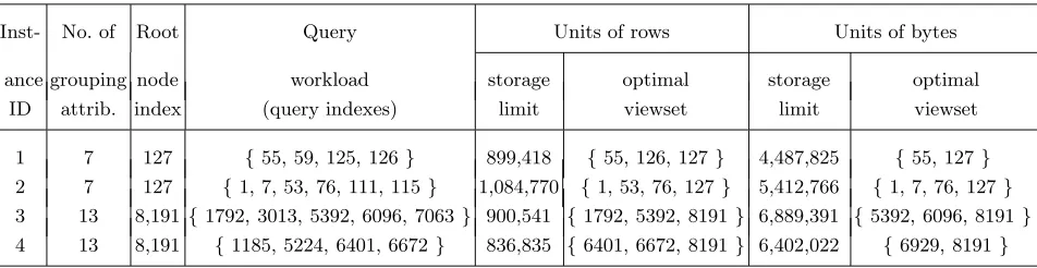
5.4 Measuring Table Sizes in Rows and Bytes
In another set of experiments we used bytes, rather than rows, to measure view sizes. View
sizes and query costs are typically measured in units of rows (see, e.g., [18, 20, 31]). At the
costs in database-management systems, because the cost of answering a query using a view
is proportional to the number of disk blocks occupied by the view. In some experiments we
expressed in bytes both the storage requirements for the views and the costs of answering
queries using those views. Note that if we state the problem this way for units of bytes, we
do not need to change the formulation (equalities and constraints) of our IP model.
Inst- No. of Root Query Units of rows Units of bytes
ance grouping node workload storage optimal storage optimal ID attrib. index (query indexes) limit viewset limit viewset
1 7 127 {55, 59, 125, 126} 899,418 {55, 126, 127} 4,487,825 {55, 127}
2 7 127 {1, 7, 53, 76, 111, 115} 1,084,770 {1, 53, 76, 127} 5,412,766 {1, 7, 76, 127}
3 13 8,191 {1792, 3013, 5392, 6096, 7063} 900,541 {1792, 5392, 8191} 6,889,391 {5392, 6096, 8191}
4 13 8,191 {1185, 5224, 6401, 6672} 836,835 {6401, 6672, 8191} 6,402,022 {6929, 8191}
Table 2.Solving the problem for units of rows and bytes.
In our experiments, for some problem instances we obtained identical optimal solutions
when view sizes and query costs are measured in rowsandbytes; for other instances, however,
we obtained different results. In Table 2 we report some results where we obtained different
optimal solutions when we used units of rows versus units of bytes. The table shows
exper-imental results for two problem instances on a view lattice with seven grouping attributes
(instance IDs 1 and 2), and for two problem instances on a view lattice with thirteen
group-ing attributes (instance IDs 3 and 4); the raw-data view for each lattice comes from the
TPC-H dataset [36]. For each instance we report the ID of the root node of the lattice; the
root node is the raw-data view, which is (similarly to [20]) always required to be part of the
For each of the four problem instances we did two experiments — one with the storage
limit and all view sizes measured in rows, and the other with the storage limit and view sizes
measured in bytes. For example, the second row of Table 2 gives results for two experiments
for instance ID 2. One experiment was done for the value of storage limitb= 1,084,770 rows,
and the other was done for b = 5,412,766 bytes. (We set the value of b in units of rows and
of bytes in such a manner that the instances are comparable.)
Our main observation on the results in Table 2 is that regardless of the units employed
(rows or bytes), the IP model that we propose can be used to obtain an optimal solution
for the problem within a reasonable amount of execution time (less than 20 seconds for the
instances reported earlier), and using the units of bytes in this context does not impose any
additional computational burden for solving the IP model. Further, the two optimal solutions
obtained when we use these units of measurement are not necessarily identical. As units of
bytes (instead of rows) is a more realistic measure in the context of view selection, we posit
that these units should be employed as the primary units of measurement in problem inputs.
5.5 Solving the OV I P0 Problem
We now outline our experimental results for the OV IP0
version of the problem, where the
top raw-data view in a view lattice is not required to be materialized. This version of the
problem can arise in, for instance, data warehouses with form interfaces, where the total
number of parameterized queries that a user can ask is finite and fixed by the interface.
Another application is situations where it may be too expensive to maintain the raw-data
be materialized; these situations include data-integration settings where certain views are
materialized in the mediator to improve query-processing efficiency [19]. (Recall that in
many cases, the top raw-data view in the view lattices of [20] is the result of joining several
base relations in the star schema.) Note that even though in this paper we compare our
approach to the heuristic approach HHRU of [20] (see Section 6), we could not do the
comparison in this setting as theHHRU approach requires that the raw-data view be always
materialized. Clearly the optimal cost for OV IP0
can be smaller than the optimal cost for
the correspondingOV IP since in OV IP0
we are not forced to materialize the raw-data view.
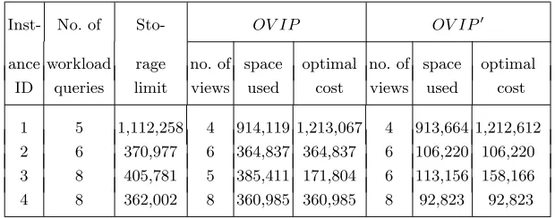
We report here some representative problem instances and solutions for a 7-attribute
TPC-H dataset, with relation sizes measured in rows. In Table 3, the value of the storage
limit for each problem instance is the sum of the size of the raw-data view with .67 the
sum of the sizes of the answers to the input queries. By “optimal cost” (columns 6 and 9 in
Table 3) we denote the total cost of evaluating the input queries using our optimal solutions.
Inst- No. of Sto- OV IP OV IP0
ance workload rage no. of space optimal no. of space optimal ID queries limit views used cost views used cost
1 5 1,112,258 4 914,119 1,213,067 4 913,664 1,212,612 2 6 370,977 6 364,837 364,837 6 106,220 106,220 3 8 405,781 5 385,411 171,804 6 113,156 158,166 4 8 362,002 8 360,985 360,985 8 92,823 92,823
Table 3.Solving theOV IP andOV IP0problems.
For example, in instance 2 in Table 3 we solved the problem for six queries, with IDs
{40,50,52,88,104,112}. The storage limit for both the OV IP and OV IP0
versions of the
IDs{40,50,52,127,104,112}; the first view (ID 40) is used to answer the first query (ID 40), the second view (ID 50) is used to answer the second query (ID 50) and so on. Note that
the raw-data view 127 is used to answer query 88. The resulting storage-space requirement
for OV IP is 364,837 tuples, and the solution cost is also 364,837. (Here, the storage-space
requirement for the solution is the same as the solution cost because each view is used
to answer a distinct workload query.) In the OV IP0
version of the problem, we obtained
six views with IDs {40,50,52,120,104,112}. The resulting storage-space requirement and solution cost for OV IP0
are both 106,220. (This solution for OV IP0
, while not identical
to the input query workload, is still globally optimal for this problem instance, because the
query-evaluation costs of both solutions are identical on the problem inputs.)
In Table 3 we see that the solution cost is consistently lower for the OV IP0
version of
the problem (column 9) than for the OV IP version (column 6) — even when the number of
materialized views is greater in theOV IP0
version (see instance 3 in Table 3, columns 4 and
7). The storage space actually used by the solutions (columns 5 and 8) gives an intuition for
why the costs are the way they are — recall that the cost of answering each workload query
is the size, in rows, of the smallest-size view that can be used to answer the query.
6
Comparing
OV I P
to the Leading Heuristic Procedure
In order to further evaluate our proposed approach for solving the view-selection problem,
we have experimentally compared the effectiveness of the approach with that of a leading
greedy construction, was proposed in Harinarayan et al. [20]; throughout this section we refer
to it as procedureHHRU. (See Appendix A in [6] for the details ofHHRU.) In this section
we discuss our experimental study and present the findings. Briefly stated, our empirical
observations are as follows:
– The execution time required for solving OV IP is generally smaller than the execution
time required by HHRU; this implies that we can solve larger instances of the problem
via OV IP than we can via HHRU.
– In some instances the quality of the solution obtained viaHHRU is comparable to (either
close to or identical with) the optimal solution obtained via OV IP. However, in other
instances the quality of the solution obtained viaHHRU is far from the optimal solution.
We also demonstrate that in general the value of the solution obtained via HHRU can
be significantly larger than the optimal value. To this end we present a family of problem
instances for which the performance ratio for the heuristic procedure (defined as the value
of the solution obtained viaHHRU divided by the optimal value) can be arbitrarily large.
6.1 Computational Results and Empirical Observations
To carry out this comparative study, we developed an independent computer program for
the heuristic procedureHHRU. This program is written in C and run on the same machine
that we used for solving the OV IP models, as described in Section 5.
The data sets that we used to carry out the experiments were the same as those described
observations that we report in this section pertain to these instances. We ran a similar
experiment in which we used the units of bytes to measure the view sizes. We noticed that
the pattern of our observations did not change in any significant manner, except that when we
used bytes to measure view sizes, in those instances where HHRU did not find the optimal
solution, the difference between the value obtained by HHRU and the optimal value was
slightly larger (at the order of 1% or 2%). In all instances that we report, unless specifically
mentioned otherwise, we set the value of the storage limit to the size of the top raw-data
view plus half the sum of sizes of the answers to the input queries.
On the TPC-H dataset, we solved instances with 7, 13, 15, and 17 attribute lattices. The
results that we present primarily pertain to the 7-attribute lattice. Our observations with the
13- and 15-attribute lattices were similar, except that the execution time was generally larger.
In the case of the 17-attribute lattice, however, for most instances that we attempted to solve
via the IP model the corresponding execution time was larger than the 15-minute time limit
that we imposed, hence we terminated the algorithm prior to its successful completion. Only
in a few such instances the algorithm terminated successfully within the imposed time limit,
and in all these instances it actually terminated very quickly (within 3 seconds). In contrast,
when we attempted to solve a similar set of instances viaHHRU we did not succeed to solve
even one such instance, due to its excessive computation time.
Within each lattice we constructed and solved several problem instances using both the
OV IP model and the HHRU procedure. Each instance has a different number of input
nodes in the lattice (e.g., among all 128 nodes in the 7-attribute lattice). The set of instances
where we selected the input queries systemically includes the following special cases:
– the input queries have an ancestor-descendant relationship with each other;
– the input queries form a single path, that is, for each queryQ in the list of input queries,
each remaining query in the list is either a descendant or an ancestor of Q;
– the list of input queries consists of the entire collection of views (nodes) in the lattice.
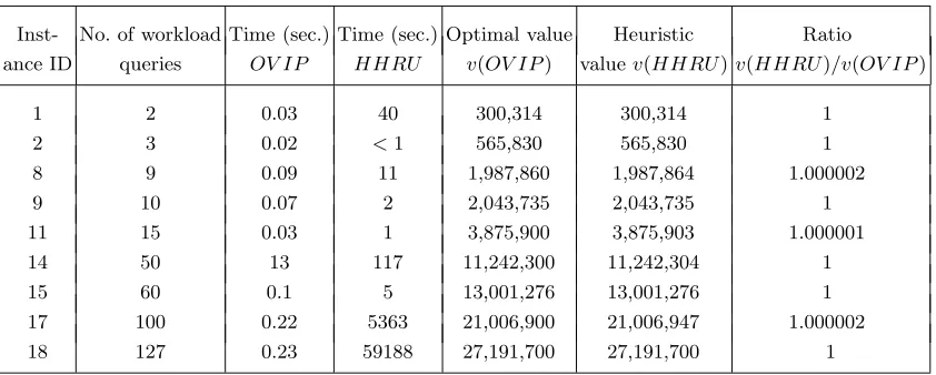
Results for nine representative instances on the 7-attribute lattice are reported in
Ta-ble 4. Results for other instances within the lattice of size 7, as well as for the instances
in other lattices, are similar to those presented here (see [6] for experimental results on all
18 instances.) For each instance in Table 4 we report the number of queries in the input
query workload, the execution time required for solving the OV IP model, the execution
time required by the HHRU procedure, the optimal value obtained via the OV IP model,
and the value of the solution obtained via the HHRU procedure. (By “value” we mean the
total cost of evaluating the workload queries using the solution output by either procedure.)
Inst- No. of workload Time (sec.) Time (sec.) Optimal value Heuristic Ratio ance ID queries OV IP HHRU v(OV IP) valuev(HHRU)v(HHRU)/v(OV IP)
1 2 0.03 40 300,314 300,314 1
2 3 0.02 <1 565,830 565,830 1
8 9 0.09 11 1,987,860 1,987,864 1.000002
9 10 0.07 2 2,043,735 2,043,735 1
11 15 0.03 1 3,875,900 3,875,903 1.000001
14 50 13 117 11,242,300 11,242,304 1
15 60 0.1 5 13,001,276 13,001,276 1
Based on these data we make two observations. First, the execution time of HHRU is
generally larger than the time for the correspondingOV IP model. Except for instance 14, the
execution time for theOV IP model is always less than one second, but the execution time for
HHRU is usually larger and varies in an unpredictable manner. One possible explanation
for this behavior of HHRU is as follows. HHRU selects one materialized view in each
iteration in a greedy manner, and terminates as soon as the total size of all materialized
views becomes close to the storage capacity b. If at an early iteration a relatively large-size
view is selected,HHRU would terminate sooner than in the case where all selected views in
the early iterations are relatively small in size. As a result, the number of input queries has a
relatively low impact on the execution time ofHHRU, while the relative size of the storage
capacity and the choice (i.e., size) of the materialized view could play a more significant role.
Our second observation is that for this collection of instances, the quality of the solutions
obtained via theHHRU procedure is relatively good. In 13 of the 18 instancesHHRU finds
an optimal solution, while in the remaining 5 instances the value of the solution found by
HHRU is within a fraction of percentage of the optimal value. But this characteristic is
not shared among all instances that we solved. In some instances the quality of the solution
obtained via HHRU was in fact far from optimal, as we discuss later in this section.
With respect to the execution time, we observed a similar behavior when we solved
numerous other instances of the problem, on 7-, 13- or 15-attribute lattices. For instances
on the 13-attribute lattice, the execution time for the corresponding OV IP model ranged
20 input queries), while the execution time for HHRU on the same instances ranged from
2 seconds (for an instance with 2 input queries) to 265 seconds (for an instance with only
10 input queries). Comparable numbers when we used OV IP to solve randomly generated
instances on the 15-attribute lattice range from 0.05 seconds (for an instance with 2 input
queries) to 3.52 seconds (for an instance with 20 input queries). On the same lattice it took
HHRU 597 seconds to solve an instance with only 2 input queries. The largest instance of
the problem that we solved using OV IP is on a 17-attibute lattice (with 15 input queries),
and it took about 2.64 seconds. In general in our experiments, the overall computational
requirements for solving the OV IP model were significantly less than those for HHRU. As
a result, we are able to solve larger instances of the problem using our proposed IP approach.
With respect to the quality of solutions obtained via HHRU we had mixed observations,
while, of course, the solutions obtained viaOV IP were consistently optimal for all instances.
Similar to the results that we presented above, we observed in many other instances that
the value of the solution obtained via HHRU is either identical to the optimal value or very
close to it. But this behavior was not consistent among all instances. Indeed in one instance
on the 7-attribute lattice the value of the solution obtained viaHHRU (i.e.,v(HHRU)) was
as much as 584 folds larger than the corresponding optimal value (i.e., v(opt)) obtained via
OV IP. See Table 5 for detailed information regarding several instances for the 7-attribute
lattice where the HHRU procedure performed poorly.
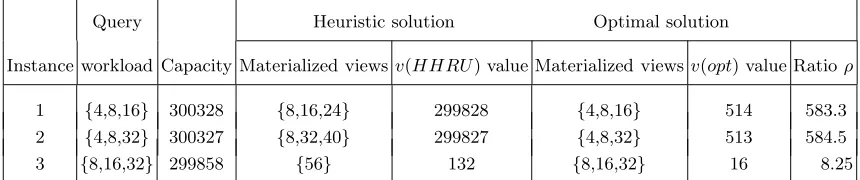
Upon further scrutiny we noticed that all instances in which HHRU performed poorly
Query Heuristic solution Optimal solution
Instance workload Capacity Materialized views v(HHRU) value Materialized viewsv(opt) value Ratioρ
1 {4,8,16} 300328 {8,16,24} 299828 {4,8,16} 514 583.3 2 {4,8,32} 300327 {8,32,40} 299827 {4,8,32} 513 584.5 3 {8,16,32} 299858 {56} 132 {8,16,32} 16 8.25
Table 5.Some instances on a 7-attribute TPC-H lattice in whichHHRUperformed poorly; root node 127 is included
in all solutions; “ratio”ρ=v(HHRU)/v(opt).
with a common parent. This led us to construct a general family of instances for which
we can show that HHRU always performs poorly relative to the globally optimal solution
returned by OV IP. We present this family of instances in the next subsection.
6.2 A Family of Instances with Special Structure
We present a family of instances of the view-selection problem for which we can demonstrate
that the quality of the solution returned by the HHRU algorithm would always be highly
suboptimal. Consider a k-attribute lattice and suppose the list of input queries includes two
queries (nodes) where each query is grouped by one attribute only; further let us assume that
these two nodes have a common parent node. We refer to these two queries as queriesq1 and
q2, respectively, and to their common parent as query p. Let c1 and c2 denote the sizes ofq1
and q2, respectively, and let cp denote the size of their common parent. Also let ctop denote
the size of the top raw-data view. For convenience of presentation we assume that queriesq1
and q2 are the only required (input) queries, although this assumption can be easily lifted
with minor adjustments (i.e., the list of input queries can include other queries as well.)
2(ctop − cp) > ctop − c1(5)
2(ctop − cp) > ctop − c2 (6)
cp > c1 + c2 (7)
The storage capacity (limit) is b=ctop + cp.
top view
parent view p
input query q1
input query q2
Fig. 7.Special-structure queries.
Under these restrictions, HHRU would select to materialize the node pbefore selecting
the node for either q1 or q2, due to Equations (5) and (6). As soon as p is selected, the
storage limit b is reached, hence the procedure terminates. The value of this solution is
v(HHRU) = 2cp, as both q1 and q2 would be evaluated using the materialized view p.
From Equation (7) it follows that the optimal solution in this case is to select nodes q1
andq2, with a total value ofv(opt) = (c1 + c2).The corresponding value of the performance
ratio isρ=v(HHRU)/v(opt) = 2cp/(c1+c2).Note that Equations (5) and (6) are equivalent
to ctop > 2cp − c1 and ctop >2cp − c2, respectively. This implies that we may select the values ofc1, c2, cp, andctop in such a manner that they satisfy all above requirements while
making the value of ρ as large as desired. This family of instances demonstrates that the
solution obtained via HHRU may be far from the optimal value (obtained via OV IP).
7
Conclusions and Future Work
We studied the following view-selection problem: Given a set of queries, a database, and an
upper bound on the amount of disk space that can be used to store materialized views, return
and reduce the evaluation costs of the queries. We focused on practically important
range-aggregate queries on star-schema data warehouses. We described an IP model that allows
us to obtainoptimal solutions without having to enumerate all possible candidate solutions.
We presented the formulation of the IP model and introduced an LP relaxation. The results
of our extensive experiments show the practicality of our approach for problem instances of
realistic sizes. We experimentally compared our method with a leading heuristic approach
in the field [20], and provided a theoretical analysis of its worst-case performance.
To solve larger instances, we are investigating techniques for developing an algorithm
that takes advantage of the special structure of the problem. Solving even larger instances of
the problem using exact methods might prove to be altogether too time consuming; thus, we
may have to use a heuristic procedure that would exploit the structure of OV IP (OV IP0
),
such as a Lagrangean heuristic [8, 26]. In addition, we are working on extending our approach
to selecting indexes alongside views, in the setting of [18], and are studying the view- and
index-selection problems under the maintenance-cost constraint on views and indexes.
References
1. F. Afrati and R. Chirkova. Selecting and using views to compute aggregate queries. InProc. ICDT, 2005.
2. S. Agarwal, R. Agrawal, P. Deshpande, A. Gupta, J.F. Naughton, R. Ramakrishnan, and S. Sarawagi. On the
computation of multidimensional aggregates. InProc. VLDB, pages 506–521, 1996.
3. S. Agrawal, S. Chaudhuri, and V.R. Narasayya. Automated selection of materialized views and indexes in SQL
databases. InProc. VLDB, pages 496–505, 2000.
4. S. Agrawal, S. Chaudhuri, and V.R. Narasayya. Materialized view and index selection tool for Microsoft SQL
5. Z. Asgharzadeh Talebi, R. Chirkova, and Y. Fathi. Experimental study of an IP model for the view selection
problem. Technical Report TR-2005-34, NCSU, July 2005.
6. Z. Asgharzadeh Talebi, R. Chirkova, and Y. Fathi. A study of a formal model for view
selection for aggregate queries. Technical Report TR-2006-2, NCSU, 2006. Available from
http://dbgroup.ncsu.edu/rychirko/Papers/techReport010506.pdf.
7. E. Baralis, S. Paraboschi, and E. Teniente. Materialized view selection in a multidimensional database. InProc.
VLDB, 1997.
8. J. Barcelo and J. Casanovas. A heuristic Lagrangean algorithm for the capacitated plant location problem.
European Journal of Operations Research, 15:212–226, 1984.
9. S. Chaudhuri and U. Dayal. An overview of data warehousing and OLAP technology.SIGMOD Record, 26:65–74,
1997.
10. S. Chaudhuri, R. Krishnamurthy, S. Potamianos, and K. Shim. Optimizing queries with materialized views. In
Proc. ICDE, pages 190–200, 1995.
11. S. Chaudhuri and V.R. Narasayya. AutoAdmin ’What-if’ index analysis utility. InProc. ACM SIGMOD, 1998.
12. R. Chirkova, A.Y. Halevy, and D. Suciu. A formal perspective on the view selection problem. VLDB Journal,
11(3):216–237, 2002.
13. S. Cohen, W. Nutt, and A. Serebrenik. Rewriting aggregate queries using views. InProc. PODS, 1999.
14. G. Cornuejols, G.L. Nemhauser, and L.A. Wolsey. The uncapacitated facility location problem. Technical Report
605, Operations Research and Industrial Engineering, Cornell University, 1984.
15. R. Fourer, D.M. Gay, and B.W. Kernighan. AMPL: A Modeling Language for Mathematical Programming. Boyd
and Fraser, Danvers, Mass., 2002.
16. J. Gray, S. Chaudhuri, A. Bosworth, A. Layman, D. Reichart, and M. Venkatrao. Data cube: A relational
aggregation operator generalizing Group-by, Cross-Tab, and Sub Totals. Data Mining and Knowledge Discovery,
1(1):29–53, 1997.
17. A. Gupta, V. Harinarayan, and D. Quass. Aggregate-query processing in data warehousing environments. In
Proc. VLDB, pages 358–369, 1995.
18. H. Gupta, V. Harinarayan, A. Rajaraman, and J.D. Ullman. Index selection for OLAP. InProc. ICDE, 1997.
19. Alon Y. Halevy. Answering queries using views: A survey. VLDB Journal, 10(4):270–294, 2001.
21. IBM. Autonomic Computing. http://www.research.ibm.com/autonomic/.
22. R. Kimball and M. Ross. The Data Warehouse Toolkit (second edition). Wiley Computer Publishing, 2002.
23. Y. Kotidis and N. Roussopoulos. DynaMat: A dynamic view management system for data warehouses. InProc.
SIGMOD, 1999.
24. J. Krarup and P.M. Pruzan. The simple plant location problem: Survey and synthesis. European Journal of
Operations Research, 12:36–81, 1983.
25. J. Li, Z. Asgharzadeh Talebi, R. Chirkova, and Y. Fathi. A formal model for the problem of view selection for
aggregate queries. InProc. ADBIS, 2005.
26. John M. Mulvey and Harlan P. Crowder. Cluster analysis: An application of lagrangian relaxation. Management
Science, 25:329–340, 1979.
27. R. G. Parker and R.L. Rardin. Discrete Optimization. Academic Press, 1988.
28. Microsoft Research. AutoAdmin Project. http://research.microsoft.com/dmx/autoadmin/default.asp. 29. ILOG S.A. CPLEX 7.0 software package. http://www.ilog.com, 2000.
30. Dennis Shasha and Philippe Bonnet.Database Tuning: Principles, Experiments, and Troubleshooting Techniques.
Morgan Kaufmann, 2002.
31. A. Shukla, P. Deshpande, and J.F. Naughton. Materialized view selection for multidimensional datasets. InProc.
VLDB, pages 488–499, 1998.
32. K. Spielberg. Algorithms for the simple plant location problem with some side constraints. Operations Research,
17:85–111, 1969.
33. D. Srivastava, S. Dar, H.V. Jagadish, and A.Y. Levy. Answering queries with aggregation using views. InProc.
VLDB, pages 318–329, 1996.
34. A.S. Szalay, J. Gray, A.R. Thakar, P.Z. Kunszt, T. Malik, J. Raddick, C. Stoughton, and J. vandenBerg. The
SDSS SkyServer - Public access to the Sloan Digital Sky Server data. Technical Report MSR-TR-2001-104,
Microsoft Research, Microsoft Corporation, 2002.
35. D. Theodoratos and T. Sellis. Data warehouse configuration. InProc. VLDB, 1997.
36. TPC-H:. TPC Benchmark H (Decision Support). http://www.tpc.org/tpch/spec/tpch2.1.0.pdf. 37. Jennifer Widom. Research problems in data warehousing. InProc. CIKM, 1995.
38. J. Yang, K. Karlapalem, and Q. Li. Algorithms for materialized view design in data warehousing environment.