R E S E A R C H
Open Access
A residual range cell migration correction
algorithm for bistatic forward-looking SAR
Wei Pu
*, Yulin Huang, Junjie Wu, Jianyu Yang and Wenchao Li
Abstract
For bistatic forward-looking synthetic aperture radar (BFSAR), images are often blurred by uncompensated radar motion errors. To get refocused images, autofocus is a useful postprocessing technique. However, a severe drawback of the autofocus algorithms is that they are only capable of removing one-dimensional azimuth phase errors. In BFSAR, motion errors and approximations of imaging algorithms introduce residual range cell migration (RCM) on BFSAR data as well. When residual RCM is within a range resolution cell, it can be neglected. However, the residual migration, which exceeds a range cell, is increasingly encountered as resolution becomes finer and finer. A novel residual RCM correction method is proposed in this paper. By fitting the low-frequency phase difference of adjacent azimuth cells, residual RCM of each azimuth cell can be corrected precisely and effectively. Simulations and real data experiments are carried out to validate the effectiveness of the proposed method.
Keywords: Bistatic forward-looking synthetic aperture radar (BFSAR), Residual range cell migration (RCM), Low-frequency fitting
1 Introduction
Forward-looking imaging is highly desirable in some applications, such as airplane navigation and landing. Due to the ability to obtain high-resolution image of the forward-looking terrain, bistatic synthetic aperture radar (SAR) is drawing more and more attention in recent years. However, the moving platforms introduce relative motion between radars and observed scene, which induces range cell migration (RCM) to bistatic forward-looking SAR data. The procedure of RCM correction is essential for the frequency domain imaging algorithms.
Usually, RCM cannot be corrected completely in prac-tical application. The reason is that there are some resid-ual components, namely residresid-ual RCM. And the residresid-ual RCM is introduced by motion errors [1]. In the pre-sumption that residual RCM is within a range resolution cell, residual RCM can be neglected [2, 3], and motion errors can be compensated by autofocus methods com-pletely. Generally speaking, residual RCM is relatively small and can be neglected in monostatic SAR, while the unique characteristics of BFSAR makes the residual RCM
*Correspondence: [email protected]
Department of Electronic Engineering, University of Electronic Science and Technology of China, 2006 Xiyuan Road, Gaoxin Western District, 611731 Chengdu, China
exceeding range resolution cell inevitable. On the one hand, the separated platforms of BFSAR induce motion errors much larger than the errors in monostatic SAR raw data. On the other hand, the higher order terms of range migration are always neglected in BFSAR imaging algorithms. However, the impacts of these higher order terms become serious when the squint angle gets larger and the resolution gets higher. In this situation, resid-ual RCM correction becomes a necessary procedure for BFSAR imaging. In principle, it is possible to compute the residual RCM from orbit and attitude data provided by an ancillary instrument such as inertial measurement units (IMU) and global positioning system (GPS). Nev-ertheless, measurement uncertainties on the data would limit the accuracy, and the data remains unknown for some unmanned aerial vehicles without ancillary instru-ment. Thus, residual RCM correction based on SAR data is indispensable.
To correct residual RCM based on SAR data, three alter-native strategies are available. (1) Estimate the azimuth phase error term firstly, and then calculate the resid-ual RCM from the estimated azimuth phase error [4]. In [4], the range compressed data is processed to a new coarser range resolution so that the presumption of aut-ofocus is met. Therefore, the azimuth phase errors can
be obtained using autofocus method from the new range compressed data and then the residual RCM can be cal-culated and compensated. However, as the azimuth phase errors are estimated in coarse resolution, the estimation precision of azimuth phase errors and residual RCM can-not satisfy the demands of high-resolution BFSAR. (2) Estimate residual RCM by making use of the relation-ship between azimuth phase errors and residual RCM. Mao et al. [3] deduces an accurate analytical relation-ship between azimuth phase errors and residual RCM in spotlight SAR. Using this relationship, a 2-D autofocus method, which can compensate the azimuth phase errors and residual RCM simultaneously, is proposed. Neverthe-less, this relationship is valid just in the case of spotlight SAR data, so that applicability of this method is limited. (3) Estimate the residual RCM independently. The resid-ual RCM correction method proposed in [5] is based on range alignment algorithm which is utilized in transla-tional motion compensation on inverse SAR (ISAR)[6, 7]. However, parametric model of the range displacement in [6] restricts the estimation accuracy, and the interpolation procedure in [7] requires exhaustive computation.
In [8], a novel residual RCM correction algorithm based on low-frequency fitting is proposed for monostatic SAR to correct the motion-induced errors. In this paper, this residual RCM correction algorithm is greatly improved to cope with BFSAR data. By estimating the residual RCM utilizing the least-squares method in the low-frequency area and compensating the displacement in frequency domain, a sub-pixel level correction result can be achieved in this proposed method. Compared with previous works on residual RCM correction of SAR data, the proposed method can realize residual RCM correction with accu-racy of sub-pixel level but requiring neither interpolation nor parametric model. Compared with [8], the novelty of the proposed method in this paper includes two parts. Firstly, a phase difference denoising procedure is added to make the proposed method more robust and can be adapted to the practical condition. Secondly, the one iso-lated dominant target assumption is not indeed needed for the proposed method, which makes the proposed method can be widely used in most practical condition. Furthermore, the range curvature term and even higher order terms, which is the unique problem in BFSAR, also can be solved by the proposed method. Simulation and real BFSAR data-processing results are presented to verify the effectiveness of the proposed method.
2 Problem formulation
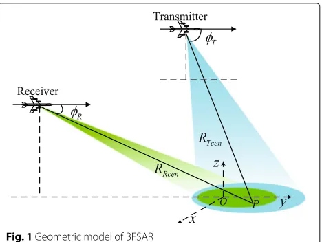
The geometric model in Fig. 1 provides the basis for BFSAR imaging. In the ideal condition, the transmitter and receiver are moving along parallel tracks with equal velocity. The squint anglesφT andφR and initial ranges
RTcen and RRcen shown in Fig. 1 are measured at the
Fig. 1Geometric model of BFSAR
composite beam center crossing time of the reference targetP.
Assume that linear frequency modulated (LFM) pulses are transmitted by the radar. The demodulated signal from the reference target in the presence of motion errors can be adequately described by
s(τ,t)=rect
τ− ¯R(t)/c Tr
rect
t Ta
×exp
−jπKr
τ− R¯(t)
c
2
×exp
−j2πR¯(t)
λ (1)
whereKris the transmitted chirp rate,Tris the timewidth of the LFM pulse, andTais the synthetic aperture time. The range time is given by τ, and t denotes the cross-range time, λ is the wavelength, and c is the speed of propagation.
In (1),R¯(t)is the instantaneous two-way range of refer-ence target P in the presrefer-ence of motion errors.R¯(t)can be formulated as
¯
R(t)=R(t)+δR(t) (2)
where δR(t) denotes the instantaneous range displace-ment induced by motion errors, andR(t)represents the nominal instantaneous two-way range.
R(t)=
R2Tcen+(Vt)2−2RTcenVtcosφT
Expand (3) att= 0 to its Taylor series andR(t)can be rewritten as
R(t)=RTcen+RRcen
−(VcosφR+VcosφT)t
+
V2sin2φR 2RRcen +
V2sin2φT 2RTcen
t2+ · · · (4)
The linear and quadratic terms in (4) are called the range walk and range curvature, respectively. In BFSAR, the total range cell migration (RCM) is dominated by the range walk component [9]. Usually, linear RCM cor-rection (LRCMC) procedures in azimuthal time domain like squint minimization [10] and keystone transform [11] are utilized to correct the range walk. After range compression and LRCMC, a coarse range focusing signal s(τ,t)is obtained.
s(τ,t)=sinc
τ− RTcen+RRcen
c −
R(t) c
rect
t Ta
exp
−j2π
λ R¯(t)
(5)
whereR(t)in the range profile is
R(t)=δR(t)+
V2sin2φ R 2RRcen +
V2sin2φ T 2RTcen
t2+ · · ·
(6)
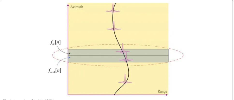
In (5), the displacementR(t)/cin the range profile is residual RCM. To illustrate the influence of residual RCM, the simple sketch map of residual RCM is shown in Fig. 2.
In Fig. 2, the solid line denotes the migration trajectory of a prominent scatter after range compression and range cell migration.
The nonlinear migration trajectory in Fig. 2 is intro-duced by residual RCM. When the residual RCM exceeds a range resolution, 2-D defocus will emerge in the final image. The reason is that the energy of target scatter dif-fuses in several range cells and induces image defocus in range direction. Besides, the general presumption of aut-ofocus is not valid, and there is considerable challenge for autofocus methods. When the autofocus procedures are performed in the azimuth direction, the azimuth signal is assumed to be a LMF signal. While in the condi-tion that the residual RCM exceeds a range resolucondi-tion, the energy of one target scatter diffuses in several range cells. Thus, the azimuth signal in a given range bin is not a complete LFM signal any more. Autofocus meth-ods can not be correctly utilized as for a incomplete LFM signal. Hence, autofocus techniques are not effec-tive if the residual errors are larger than range cell. And therefore, the image results defocus in azimuth direction as well.
Therefore, in order to obtain high-resolution BFSAR image, residual RCM correction is essential.
3 Residual RCM correction
In this section, a novel residual RCM correction method is proposed. Residual RCM of each azimuth cell is corrected one by one. Here, the residual RCM correction method for one azimuth cell is presented in the rest of this section.
3.1 Row correlation analysis
Letfm[n] andfm+1[n] denote the adjacent azimuth cells of BFSAR data as shown in Fig. 2, wherem=1, 2,· · ·,M
indexes the transmitted pulses andn=1, 2,· · ·,Nstands for the samples taken from each pulses,Mis the azimuth sample number, andNis the range sample number.
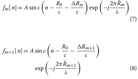
According to (5),fm[n] andfm+1[n] can be written as placement measured at themth transmitted pulse, respec-tively;R¯m+1andRm+1denote the slant range and range displacement measured at the (m+1)th transmitted pulse, respectively.
From (7) and (8), the relationship between the adjacent azimuth cellsfm[n] andfm+1[n] can be deduced.
That is to say, apart from the displacement nm+1, two adjacent rows of the data can be considered as approximately equal.
The similarity of adjacent rows can be measured by the correlation value (CV), which is defined as:
r=
whereris the correlation value of adjacent rows,
gm+1[n]=fm+1[n]
gm[n]=fm[n] (12)
In this article, it is assumed that the adjacent rows of data can be regarded as approximately equal if the aver-age CV is larger than 0.85. Fortunately, the range focused data of natural scenes collected by BFSAR system can sat-isfy this condition. Figure 3a presents the simulated range focused data with one target, and Fig. 3b depicts the cor-relation function curve of the range focused data. White Gauss noise with SNR=5 dB is added into the simu-lated data. Simulation parameters are listed in Table 1. It can be seen that the CVs meet the requirements completely.
Taking the real data of BFSAR as an example, and calcu-lating the correlation value of 10,000 group adjacent rows, respectively, we can get the correlation function curve in Fig. 4b. We carry out an airborne BFSAR experiment in 2012 [12]. The actual data comes from the experiment. It
Range(m)
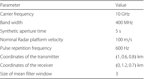
Table 1Simulation parameters
Parameter Value
Carrier frequency 10 GHz
Band width 400 MHz
Synthetic aperture time 5 s
Nominal Radar platform velocity 100 m/s
Pulse repetition frequency 600 Hz
Coordinates of the transmitter (1, 0.6, 0.8)km
Coordinates of the receiver (0, 1.2, 0.7)km
Size of mean filter window 3
is shown in Fig. 4b that due to the continuity of the scene, the CVs of adjacent rows are all above 0.87, i.e., the adja-cent rows of data can be regarded as approximately equal. It can be seen that the CVs meet the requirements as for the BFSAR data as well.
Hence, it is reasonable to regard the two adjacent rows of the data as approximately equal, and this feature pro-vides the theoretical basis for the proposed algorithm.
3.2 Phase difference extraction
According to (7), (8), and (10), we can write
Fm+1(ω)=Fm(ω)
exp
−jωnm+1−j
2πR¯m+1− ¯Rm
λ
(13)
where Fm+1(ω)andFm(ω)are the frequency spectra of
fm+1[n] and fm[n], respectively. Then, phase difference betweenFm+1(ω)andFm(ω)can be calculated by Eq. (14).
(ω)= −nm+1ω−
2πR¯m+1− ¯Rm
λ (14)
where (ω) ∈ (−π,π] denotes the phase difference betweenFm+1(ω)andFm(ω). As known to all, the phase is limited to the interval of(−π,π] and leads to the tran-sition of a phase difference from−π to π. In order to get a continuous phase difference curve, it is necessary to unwrap the phase spectrum while limited SNR of a BFSAR data can result in a great difference between adja-cent rows of data. Hence, there will be a large local jitter in the phase difference curve, which will lead to failure of phase unwrapping. As a result, the number of fitting points to a linear function would decrease. Therefore, the phase difference curve should be denoised and smoothed before unwrapping.
3.3 Phase difference denoising
A median filter or a mean filter can not be simply applied into the denoising of phase, because they would seriously destroy the transition property in the phase difference spectrum. Let [n] denote the discrete version of the (ω). Consider the phase sequence
a[n]=cos( [n]) (15) b[n]=sin( [n]) (16)
The formulas mentioned above make the original phase [n] transform into the continuous sine/cosine phase sequence a[n] and b[n], which then can be filtered by the mean filter as
Range (Samples)
Azimuth (Samples)
500 1000 1500 2000 2500
1000
2000
3000
4000
5000
6000
7000
8000
9000
10000
(a)
0 1000 2000 3000 4000 5000 6000 7000 8000 9000 10000 0.88
0.9 0.92 0.94 0.96 0.98
CVs
Azimuth (Samples)
(b)
¯
a[n]= 1 M
i∈W
a[n] (17)
¯
b[n]= 1 M
i∈W
b[n] (18)
whereW is the neighborhood with centernandMis the size of mean filter window. In the phase difference curve, the jitter at some locations is large, while other locations are relatively flat. Therefore, the size of the mean filter window M can not be a constant value, but should change with a specific parameter. When the jitter is large, a small window should be used; otherwise, it is likely to make the curve too flat. When the jitter is flat, a larger win-dow should be used, which makes the curve as smooth as possible. Calculate the arctangent function through the filtered sin/cosine values as
1[n]=arctan
¯
b[n]
¯
a[n] (19)
By using the arctangent function as inverse mapping, the filtered sawtooth phase is limited in the interval of (−π/2,π/2]. By judging the quadrant of the phase differ-ence sequdiffer-ence through the positive and negative relation-ship between sine and cosine values, the filtered smooth phase difference sequence can be determined. After the phase difference denoising procedure, the jitter in the phase difference decreases a lot, which makes the phase unwrapping more accurately.
In principle, the displacement nm+1 can be estimated by fitting the slope of the phase difference curve 1[n]. However, the displacement estimated at this point is inac-curate. The reason is that there exists some minute dif-ferences between two adjacent rows due to the noise
and clutter in practical application. The corresponding solution will be discussed in the next subsection.
3.4 Low-frequency fitting
Information between fm[n − nm+1] and fm+1[n] can be divided into macroscopic similarity and detailed difference, which correspond to low-frequency and high-frequency components in frequency spectrum, respectively. The low-frequency part, which corresponds to the similarity of adjacent azimuth cells, is a data seg-ment similar to the ideal phase curve, and it can be fit to a straight line. While the high-frequency part, which corre-sponds to the detailed difference of adjacent azimuth cells, cannot be fit correctly.
Therefore, taking the low-frequency spectrum informa-tion to fit the phase difference curve with the least-squares method is a feasible way precise estimation. In the fol-lowing, a strategy to select the low-frequency part is presented.
1. The first-order differential of the phase difference curve can be calculated as
[n]= 1[n]− 1[n−1] (20)
2. By using a mean filter, the derivative curve is smoothed.
ϕ[n]= 1 M
i∈W
[n], (21)
whereW is the neighborhood with center n and M is the size of mean filter window.
3. Search peaks ofϕ[n]from the central zero frequency. If the peak value is larger than the threshold, set the fitting area between zero and the peak value.
1[ ]
Fig. 6Illustration of residual RCM in the presence of two dominant targets
The differential phase difference in step 2 presents a notch area in the low-frequency part. The adjacent aver-age method in step 2 aims at reducing false positives, which means avoiding putting the jitter low-frequency points into the high-frequency points. Step 3 selects the low-frequency part by searching the notch area of differ-ential phase difference.
At this point, least-squares method is utilized to fit the slopenm+1in the low-frequency part. Then, correspond-ing correction result˜fm+1[n] can be achieved according to (22).
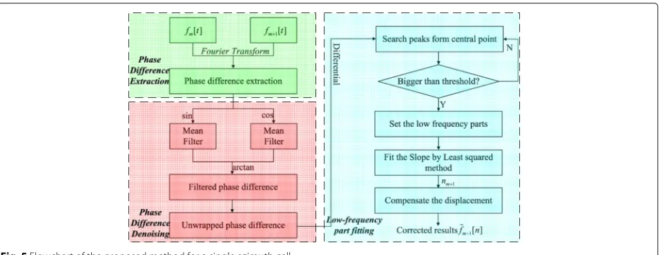
To make it clear, the flowchart of the proposed residual RCM correction method for a single azimuth cell is shown in Fig. 5.
3.5 Discussion
In the proposed method, a dominant point-target model, i.e., the presence of one strong scatterer per footprint.
Indeed, when only distributed targets are present sig-nificant decorrelation between adjacent azimuth cells is expected to appear. For example, when two dominant tar-gets are located in the scene, the signal after coarse range focusing is shown in Fig. 6.
As for the azimuth bins fm[n] andfm+1[n], there are significant decorrelation, and the relationship in Eq. (9) cannot be satisfied. In this condition, the assumption for the proposed method is not valid, and we cannot esti-mate the range deviation difference between these two range bins. In order to cope with this problem, the CV between the adjacent azimuth bins should be calculated first. Then, as for the azimuth bins that the CV is smaller than the threshold, we do not estimate the range deviation difference. After the range deviation differences of most azimuth bins are estimated, the range deviations of the azimuth bin, whose CV is smaller than the threshold, are estimated based on the range deviation difference of the adjacent azimuth bins by the fitting methods.
In addition, computational complexity of the proposed method is analyzed here. Suppose the range and azimuth samples areNr andNa, respectively. The computational complexity of the proposed residual RCM correction method for a single azimuth cell is elaborated as follows. (1) The phase difference extraction procedure uses two times Fourier transform and two times phase factor mul-tiplication. The computational complexity isO(NrlogNr). (2) The phase difference denoising procedure uses five times phase factor multiplication and one 1-D phase unwrap processing. The phase unwrap processing in [13] is utilized in this paper, and the computation complex-ity of this processing is O(Nr). As a consequence, the computation complexity of this phase difference denois-ing procedure isO(Nr). (3) The major operations of low frequency fitting procedure are three times phase factor multiplication, one time linear search, one time inverse Fourier transform, and one time linear fitting. The com-putational complexity isO(NrlogNr). As a consequence,
Range(m)
Fig. 8 aImaging results without residual RCM correction.bImaging results with residual RCM correction of MEM.cImaging results with residual RCM correction of the proposed methods
the computational complexity for the whole algorithm is O(NaNrlogNr).
4 Experimental results
In this section, both of the point target simulation and the real data experiment are performed to evaluate the performance of the proposed residual RCM correction algorithm for BFSAR.
4.1 Simulation and analysis
Some simulation parameters are shown in Table 1. Three point targets (A,O, andB) are assumed to be distributed in the scene. The coordinates of the targetsA,O, andB are(−200, 0), 0(0, 0), and(200, 0)m, respectively. Motion errors are added to the raw data of BFSAR. LetxT and xR denote the deviations in xdirection for the trans-mitter and receiver, yT andyRdenote the deviations inydirection for the transmitter and receiver, whilezT and zR denote the height deviations of the transmit-ter and receiver, respectively. Functions of these devia-tions with respect to the azimuth time t are presented in (23).
Range (Samples)
Azimuth (Samples)
20 40 60 80 100 120 140 160 200
400 600 800 1000 1200 1400 1600
Range (Samples)
Azimuth (Samples)
20 40 60 80 100 120 140 160 200
400 600 800 1000 1200 1400 1600
Range (Samples)
Azimuth (Samples)
20 40 60 80 100 120 140 160 200
400 600 800 1000 1200 1400 1600
(a) (b) (c)
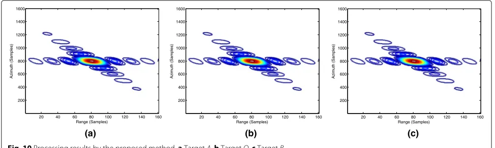
Fig. 10Processing results by the proposed method.aTargetA.bTargetO.cTargetB
After correcting the residual RCM, a robust autofocus method MIA [14] is applied to obtain the imaging results. Final compressed images of the target in the scene center are shown in Fig. 8. Quality of the image without resid-ual RCM correction suffers considerable degradation in both azimuth and range direction in Fig. 8a. In Fig. 8b, c, the imaging qualities are improved using MEM and the proposed method.
In order to compare the performance of MEM and the proposed method, the three targets in the imaging results of MEM and the proposed method are interpolated eight times as shown in Figs. 9 and 10, respectively. The results show that we can get the perfectly focused imaging results by the proposed method, while the imaging results can not be focused well by MEM. Besides, we measure the quality of imaging results of the focused targets of the proposed method and MEM by peak sidelobe ratio (PSLR), inte-grated sidelobe ratio (ISLR), and impulse-response width (IRW) as shown in Table 2. From Table 2, it also can be found that the proposed method has a better performance than MEM.
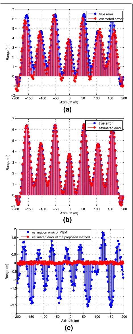
True displacement and estimated displacement are shown in Fig. 11a, b, and the estimation errors are shown in Fig. 11c. It can be seen that the estimated displace-ment matches quite well with the true displacedisplace-ment in the proposed method, and the variation of the root mean square (RMS) of an overall estimation error is 0.011 m.
Compared with the proposed method, estimation accu-racy of MEM is bad, and the RMS is 1.21 m. The reason is that the displacement estimated by MEM must be modeled as a polynomial, which restricts the estimation accuracy.
The performance of the proposed method in terms of precision and robustness to noise is evaluated. Gaussian white noise with different SNRs is added to the range compression data, and 1000 repetitions of each case were carried out. Figure 12a, b shows the RMS, calculated from simulation results, as a function of SNR by MEM and the proposed method, respectively. It is clear that if SNR is larger than 5 dB, the RMS results obtained from the pro-posed method are lower than 0.012 m. If SNR is smaller than 5 dB, the proposed method performs poorly with SNR tending to zero. The RMS of MEM increases when the SNR becomes smaller as well. Compared with the pro-posed method, the estimation results show that MEM is more sensitive to noise. Future work will study the per-formance of the proposed method in terms of robustness to noise.
4.2 Real data results
In 2012, we performed an airborne BFSAR experiment which was the first airborne bistatic forward-looking experiments in the world [12]. In this experiment, the two platforms were mounted on two airplanes of Yun-5. The
Table 2Imaging quality parameters
Range Azimuth
PSLR(dB) ISLR(dB) IRW(m) PSLR(dB) ISLR(dB) IRW(m)
Target A −13.35 −10.22 0.68 −13.19 −10.09 0.88
By the proposed Target O −13.37 −10.23 0.67 −13.26 −10.17 0.84
method Target B −13.34 −10.22 0.68 −13.14 −10.11 0.86
Target A −8.02 −7.97 0.91 −6.03 −4.76 1.98
By MEM Target O −13.37 −8.23 0.87 −6.76 −5.68 1.84
−200 −150 −100 −50 0 50 100 150 200 −2
−1 0 1 2 3 4 5 6 7
Azimuth (m)
Range (m)
true error estimated error
(a)
−200 −150 −100 −50 0 50 100 150 200
−1 0 1 2 3 4 5 6 7
Azimuth (m)
Range (m)
true error estimated error
(b)
−200 −150 −100 −50 0 50 100 150 200
−3 −2.5 −2 −1.5 −1 −0.5 0 0.5 1 1.5 2
Azimuth (m)
Range (m)
estimation error of MEM
estimated error of the proposed method
(c)
Fig. 11 aEstimation results by MEM.bEstimation results by the proposed method.cEstimation error
0 5 10 15 20 25 30
1 1.5 2 2.5 3 3.5 4 4.5 5 5.5 6
SNR(dB)
RMS(m)
(a)
0 5 10 15 20 25 30
0.01 0.015 0.02 0.025 0.03 0.035 0.04 0.045
SNR(dB)
RMS(m)
(b)
Fig. 12 aRMS of estimated residual RCM versus SNR by MEM.bRMS of estimated residual RCM versus SNR by the proposed method
antennas of the system are two horn antennas, and the overlap of the antenna footprints was guaranteed by care-ful flight planning and pilots skill. The system works in X band. The bandwidth of the transmitted chirp signal is 75 MHz. Pulse repetition frequency is 500 Hz. The veloci-ties of the two platforms were controlled to be 42 m/s. The geometry configuration is shown in Fig. 13.
Fig. 13Geometry configuration in the airborne experiment.aSide view.bVertical view
(a)
(b)
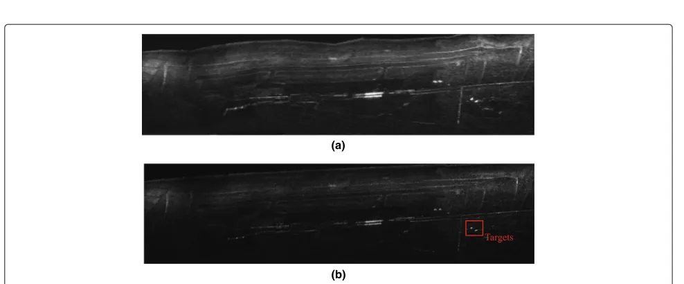
Fig. 14 aImage result without residual RCM correction.bImage result with residual RCM correction
To illustrate the detail of the proposed method, migra-tion trajectories of the targets in Fig. 14b are presented in Fig. 15. Figure 15a gives the data after range compres-sion and LRCMC. Although deterministic range migra-tion has been compensated by using RCM correcmigra-tion, residual RCM is still large enough to exceed several range resolution cells. In this situation, conventional autofocus algorithm cannot completely compensate for the errors. Figure 15b shows the imaging results utilizing MIA. It can be clearly seen that the image suffers from severely 2-D defocus.
5 Conclusions
In this paper, a novel residual RCM correction method based on low-frequency fitting for BFSAR has been proposed. By fitting the low-frequency phase difference between adjacent azimuth cells, residual RCM in each azimuth cell is corrected one by one. Using the least-squares method, the estimation result is generally not an integer, and a sub-pixel level correction result can be achieved. Compared with previous works on residual RCM correction of SAR data, the proposed method can realize residual RCM correction requiring neither inter-polation nor parametric model. In addition, the proposed algorithm is robust to noise. Simulations and experiments have been carried out to confirm the effectiveness of the proposed algorithm.
Competing interests
The authors declare that they have no competing interests.
Received: 15 March 2016 Accepted: 29 September 2016
References
1. X Mao, D Zhu, Y Zhang. Knowledge-aided two-dimensional autofocus for synthetic aperture radar. Radar Conference (RADAR) (IEEE, Ottawa, ON, 2013), pp. 1–6
2. L Yang, M Xing, Y Wang, L Zhang, Z Bao, Compensation for the NsRCM and phase error after polar format resampling for airborne spotlight SAR raw data of high resolution.Geosci. Remote Sensing Lett. IEEE.10, 165–169 (2013)
3. X Mao, D Zhu, Z Zhu, Autofocus Correction of APE and residual RCM in spotlight SAR polar format imagery. Aerospace Electron Syst. IEEE Trans.
49, 2693–2706 (2013)
4. AW Doerry,Autofocus correction of excessive migration in synthetic aperture
radar images, (US, Department of Energy, 2004)
5. JT González-Partida, P Almorox-González, M Burgos-García, BP Dorta-Naranjo, SAR system for UAV operation with motion error compensation beyond the resolution cell. Sensors.8, 3384–3405 (2008) 6. J Wang, D Kasilingam, Global range alignment for ISAR.Aerospace
electron. Syst. IEEE Trans.39, 351–357 (2003)
7. G Delisle, H Wu, Moving target imaging and trajectory computation using ISAR. Aerospace Electron. Syst. IEEE Trans.30, 887–899 (1994)
8. W Pu, J Yang, W Li, J Wu, Y Lv,A residual range cell migration correction
algorithm for SAR based on low-frequency fitting. (IEEE, Arlington, VA, 2015),
pp. 1300–1304
9. W Li, J Yang, Y Huang, J Wu, A geometry-based Doppler centroid estimator for bistatic forward-looking SAR. Geosci. Remote Sensing Lett. IEEE.9, 388–392 (2012)
10. Y Tang, B Zhang, M Xing, Z Bao, L Guo, The space-variant phase-error matching map-drift algorithm for highly squinted SAR. Geosci. Remote Sensing Lett. IEEE.10, 845–849 (2013)
11. J Wu, Z Li, Y Huang, J Yang, H Yang, QH Liu, Focusing bistatic forward-looking SAR with stationary transmitter based on keystone transform and nonlinear chirp scaling. Geosci. Remote Sensing Lett. IEEE.
11, 148–152 (2014)
12. J Yang, Y Huang, H Yang, J Wu, W Li, Z Li, X Yang. A first experiment of airborne bistatic forward-looking SAR preliminary results. Remote Sensing Symposium (IGARSS) 2013 IEEE International (IEEE, Vic., Australia, 2013), pp. 4202–4204
13. J Tribolet, A new phase unwrapping algorithm.Acoustics Speech Signal Process. IEEE Trans.25, 170–177 (1977)
14. TJ Kragh. Monotonic iterative algorithm for minimum-entropy autofocus. Adaptive Sensor Array Processing (ASAP) Workshop, (Lexington, MA, June 2006)
Submit your manuscript to a
journal and benefi t from:
7 Convenient online submission 7 Rigorous peer review
7 Immediate publication on acceptance 7 Open access: articles freely available online 7 High visibility within the fi eld
7 Retaining the copyright to your article