Complexity of Algorithms
Lecture Notes, Spring 1999
Peter G´acs
Boston Universityand
Contents
0 Introduction and Preliminaries 1
0.1 The subject of complexity theory . . . 1
0.2 Some notation and definitions . . . 2
1 Models of Computation 3 1.1 Introduction . . . 3
1.2 Finite automata . . . 5
1.3 The Turing machine . . . 8
1.4 The Random Access Machine . . . 18
1.5 Boolean functions and Boolean circuits . . . 24
2 Algorithmic decidability 31 2.1 Introduction . . . 31
2.2 Recursive and recursively enumerable languages . . . 33
2.3 Other undecidable problems . . . 37
2.4 Computability in logic . . . 42
3 Computation with resource bounds 50 3.1 Introduction . . . 50
3.2 Time and space . . . 50
3.3 Polynomial time I: Algorithms in arithmetic . . . 52
3.4 Polynomial time II: Graph algorithms . . . 57
3.5 Polynomial space . . . 62
4 General theorems on space and time complexity 65 4.1 Space versus time . . . 71
5 Non-deterministic algorithms 72 5.1 Non-deterministic Turing machines . . . 72
5.2 Witnesses and the complexity of non-deterministic algorithms . . . 74
5.3 General results on nondeterministic complexity classes . . . 76
5.4 Examples of languages in NP . . . 79
5.5 NP-completeness . . . 85
5.6 Further NP-complete problems . . . 89
6 Randomized algorithms 99 6.1 Introduction . . . 99
6.2 Verifying a polynomial identity . . . 99
6.3 Prime testing . . . 103
7 Information complexity: the complexity-theoretic notion of randomness 112
7.1 Introduction . . . 112
7.2 Information complexity . . . 112
7.3 The notion of a random sequence . . . 117
7.4 Kolmogorov complexity and data compression . . . 119
8 Pseudo-random numbers 124 8.1 Introduction . . . 124
8.2 Introduction . . . 124
8.3 Classical methods . . . 125
8.4 The notion of a psuedorandom number generator . . . 127
8.5 One-way functions . . . 130
8.6 Discrete square roots . . . 133
9 Parallel algorithms 135 9.1 Parallel random access machines . . . 135
9.2 The class NC . . . 138
10 Decision trees 143 10.1 Algorithms using decision trees . . . 143
10.2 The notion of decision trees . . . 146
10.3 Nondeterministic decision trees . . . 147
10.4 Lower bounds on the depth of decision trees . . . 151
11 Communication complexity 155 11.1 Communication matrix and protocol-tree . . . 155
11.2 Some protocols . . . 159
11.3 Non-deterministic communication complexity . . . 160
11.4 Randomized protocols . . . 164
12 The complexity of algebraic computations 166 13 Circuit complexity 167 13.1 Introduction . . . 167
13.2 Lower bound for the Majority Function . . . 168
13.3 Monotone circuits . . . 170
14 An application of complexity: cryptography 172 14.1 A classical problem . . . 172
14.2 A simple complexity-theoretic model . . . 172
14.3 Public-key cryptography . . . 173
0
Introduction and Preliminaries
0.1 The subject of complexity theory
The need to be able to measure the complexity of a problem, algorithm or structure, and to obtain bounds and quantitive relations for complexity arises in more and more sciences: besides computer science, the traditional branches of mathematics, statistical physics, biology, medicine, social sciences and engineering are also confronted more and more frequently with this problem. In the approach taken by computer science, complexity is measured by the quantity of computational resources (time, storage, program, communication) used up by a particualr task. These notes deal with the foundations of this theory.
Computation theory can basically be divided into three parts of different character. First, the exact notions of algorithm, time, storage capacity, etc. must be introduced. For this, dif-ferent mathematical machine models must be defined, and the time and storage needs of the computations performed on these need to be clarified (this is generally measured as a function of the size of input). By limiting the available resources, the range of solvable problems gets narrower; this is how we arrive at different complexity classes. The most fundamental com-plexity classes provide an important classification of problems arising in practice, but (perhaps more surprisingly) even for those arising in classical areas of mathematics; this classification reflects the practical and theoretical difficulty of problems quite well. The relationship between different machine models also belongs to this first part of computation theory.
Second, one must determine the resource need of the most important algorithms in various areas of mathematics, and give efficient algorithms to prove that certain important problems belong to certain complexity classes. In these notes, we do not strive for completeness in the investigation of concrete algorithms and problems; this is the task of the corresponding fields of mathematics (combinatorics, operations research, numerical analysis, number theory). Nevertheless, a large number of concrete algorithms will be described and analyzed to illustrate certain notions and methods, and to establish the complexity of certain problems.
Third, one must find methods to prove “negative results”, i.e. for the proof that some problems are actually unsolvable under certain resource restrictions. Often, these questions can be formulated by asking whether certain complexity classes are different or empty. This problem area includes the question whether a problem is algorithmically solvable at all; this question can today be considered classical, and there are many important results concerining it; in particular, the decidability or undecidablity of most concrete problems of interest is known.
The majority of algorithmic problems occurring in practice is, however, such that algorithmic solvability itself is not in question, the question is only what resources must be used for the solution. Such investigations, addressed to lower bounds, are very difficult and are still in their infancy. In these notes, we can only give a taste of this sort of results. In particular, we discuss complexity notions like communication complexity or decision tree complexity, where by focusing only on one type of rather special resource, we can give a more complete analysis of basic complexity classes.
be complex. These are important areas for the application of complexity theory; from among them, we will deal with random number generation and cryptography, the theory of secret communication.
0.2 Some notation and definitions
A finite set of symbols will sometimes be called analphabet. A finite sequence formed from some elements of an alphabet Σ is called a word. The empty word will also be considered a word, and will be denoted by ∅. The set of words of length n over Σ is denoted by Σn, the set of all words (including the empty word) over Σ is denoted by Σ∗. A subset of Σ∗, i.e. , an arbitrary set of words, is called alanguage.
Note that the empty language is also denoted by ∅but it is different, from the language{∅} containing only the empty word.
Let us define some orderings of the set of words. Suppose that an ordering of the elements of Σ is given. In thelexicographic orderingof the elements of Σ∗, a wordαprecedes a word β if eitherαis a prefix (beginning segment) ofβ or the first letter which is different in the two words is smaller inα. (E.g., 35244 precedes 35344 which precedes 353447.) The lexicographic ordering does not order all words in a single sequence: for example, every word beginning with 0 precedes the word 1 over the alphabet {0,1}. The increasing order is therefore often preferred: here, shorter words precede longer ones and words of the same length are ordered lexicographically. This is the ordering of {0,1}∗ we get when we write up the natural numbers in the binary number system.
The set of real numbers will be denoted byR, the set of integers byZand the set of rational numbers (fractions) byQ. The sign of the set of non-negative real (integer, rational) numbers is R+ (Z+,Q+). When the base of a logarithm will not be indicated it will be understood to be 2.
Let f and g be two real (or even complex) functions defined over the natural numbers. We write
f =O(g)
if there is a constantc >0 such that for all nlarge enough we have|f(n)| ≤c|g(n)|. We write f =o(g)
if f is 0 only at a finite number of places and f(n)/g(n) → 0 if n → ∞. We will also use sometimes an inverse of the big O notation: we write
f = Ω(g)
ifg=O(f). The notation f = Θ(g)
means that both f = O(g) and g = O(f) hold, i.e. there are constants c1, c2 > 0 such that for all n large enough we have c1g(n) ≤ f(n) ≤c2g(n). We will also use this notation within formulas. Thus,
means that (n+ 1)2 can be written in the form n2+R(n) where R(n) =O(n2). Keep in mind that in this kind of formula, the equality sign is not symmetrical. Thus, O(n) = O(nn) but O(n2) =O(n). When such formulas become too complex it is better to go back to some more explicit notation.
0.1Exercise Is it true that 1 + 2 +· · ·+n=O(n3)? Can you make this statementsharper?
♦
1
Models of Computation
1.1 Introduction
In this section, we will treat the concept of “computation” or algorithm. This concept is fundamental for our subject, but we will not define it formally. Rather, we consider it an intuitive notion, which is amenable to various kinds of formalization (and thus, investigation from a mathematical point of view).
An algorithm means a mathematical procedure serving for a computation or construction (the computation of some function), and which can be carried out mechanically, without think-ing. This is not really a definition, but one of the purposes of this course is to demonstrate that a general agreement can be achieved on these matters. (This agreement is often formulated as Church’s thesis.) A program in the Pascal (or any other) programming language is a good example of an algorithm specification. Since the “mechanical” nature of an algorithm is its most important feature, instead of the notion of algorithm, we will introduce various concepts of a mathematical machine.
Mathematical machines compute some output from someinput. The input and output can be a word (finite sequence) over a fixed alphabet. Mathematical machines are very much like the real computers the reader knows but somewhat idealized: we omit some inessential features (e.g. hardware bugs), and add an infinitely expandable memory.
Here is a typical problem we often solve on the computer: Given a list of names, sort them in alphabetical order. The input is a string consisting of names separated by commas: Bob, Charlie, Alice. The output is also a string: Alice, Bob, Charlie. The problem is to compute a functionassigning to each string of names its alphabetically ordered copy.
In general, a typical algorithmic problem has infinitely many instances, whci then have arbitrarily large size. Therefore we must consider either an infinite family of finite computers of growing size, or some idealized infinite computer. The latter approach has the advantage that it avoids the questions of what infinite families are allowed.
Historically, the first pure infinite model of computation was the Turing machine, intro-duced by the English mathematicianTuringin 1936, thus before the invention of programable
inves-tigations. It is less appropriate for the definition of concrete algorithms since its description is awkward, and mainly since it differs from existing computers in several important aspects.
The most important weakness of the Turing machine in comparison real computers is that its memory is not accessible immediately: in order to read a distant memory cell, all intermediate cells must also be read. This is remedied by the Random Access Machine (RAM). The RAM can reach an arbitrary memory cell in a single step. It can be considered a simplified model of real world computers along with the abstraction that it has unbounded memory and the capability to store arbitrarily large integers in each of its memory cells. The RAM can be programmed in an arbitrary programming language. For the description of algorithms, it is practical to use the RAM since this is closest to real program writing. But we will see that the Turing machine and the RAM are equivalent from many points of view; what is most important, the same functions are computable on Turing machines and the RAM.
Despite their seeming theoretical limitations, we will consider logic circuits as a model of computation, too. A given logic circuit allows only a given size of input. In this way, it can solve only a finite number of problems; it will be, however, evident, that for a fixed input size, every function is computable by a logical circuit. If we restrict the computation time, however, then the difference between problems pertaining to logic circuits and to Turing-machines or the RAM will not be that essential. Since the structure and work of logic circuits is the most transparent and tractable, they play very important role in theoretical investigations (especially in the proof of lower bounds on complexity).
If a clock and memory registers are added to a logic circuit we arrive at the interconnected finite automata that form the typical hardware components of today’s computers.
Let us note that a fixed finite automaton, when used on inputs of arbitrary size, can compute only very primitive functions, and is not an adequate computation model.
One of the simplest models for an infinite machine is to connect an infinite number of similar automata into an array. This way we get a cellular automaton.
1.2 Finite automata
A finite automaton is a very simple and very general computing device. All we assume that if it gets an input, then it changes its internal state and issues an output. More exactly, a finite automaton has
— an input alphabet, which is a finite set Σ,
— an output alphabet, which is another finite set Σ, and — a set Γ of internal states, which is also finite.
To describe a finite automaton, we need to specify, for every input a ∈ Σ and state s ∈ Γ, the output α(a, s) ∈Σ and the new state ω(a, s) ∈Γ. To make the behavior of the automata well-defined, we specify astarting stateSTART.
At the beginning of a computation, the automaton is in state s0 = START. The input to the computation is given in the form of a stringa1a2. . . an∈Σ∗. The first input lettera1 takes the automaton to state s1 = ω(a1, s0); the next input letter takes it into state s2 = ω(a2, s1) etc. The result of the computation is the stringb1b2. . . bn, wherebk=α(ak, sk−1) is the output at thek-th step.
Thus a finite automaton can be described as a 6-tuple Σ,Σ,Γ, α, ω, s0, where Σ,Σ,Γ are finite sets,α: Σ×Γ→Σ and ω: Σ×Γ→Γ are arbitrary mappings, and START∈Γ. Remarks. 1. There are many possible variants of this notion, which are essentially equivalent. Often the output alphabet and the output signal are omitted. In this case, the result of the computation is read off from the state of the automaton at the end of the computation.
In the case of automata with output, it is often convenient to assume that Σ contains the blank symbol∗; in other words, we allow that the automaton does not give an output at certain steps.
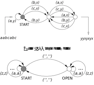
2. Your favorite PC can be modelled by a finite automaton where the input alphabet consists of all possible keystrokes, and the output alphabet consists of all texts that it can write on the screen following a keystroke (we ignore the mouse, ports, floppy drives etc.) Note that the number of states is more than astronomical (if you have 1 GB of disk space, than this automaton has something like 21010 states). At the cost of allowing so many states, we could model almost anything as a finite automaton. We’ll be interested in automata where the number of states is much smaller - usually we assume it remains bounded while the size of the input is unbounded. Every finite automaton can be described by a directed graph. The nodes of this graph are the elements of Γ, and there is an edge labelled (a, b) from state s to state s if α(a, s) = b and ω(a, s) = s. The computation performed by the automaton, given an input a1a2. . . an, corresponds to a directed path in this graph starting at node START, where the first labels of the edges on this path are a1, a2, . . . , an. The second labels of the edges give the result of the computation (figure 1.1).
(c,x)
yyxyxyx (b,y)
(a,x)
(a,y)
(b,x)
(c,y)
(a,x) (b,y)
aabcabc
(c,x)
[image:9.612.149.450.81.352.2]START
Figure 1.1: A finite automaton
...
(z,z)
(’’,’’)
...
(a,a)
(z,z)
(’’,‘‘)
(a,a)
OPEN
START
Figure 1.2: An automaton correcting quotation marks
or an odd number of ” symbols. So it will have two states: START and OPEN (i.e., quotation is open). The input alphabet consists of whatever characters the text uses, including ”. The output alphabet is the same, except that instead of ” we have two symbols “ and ”. Reading any character other than ”, the automaton outputs the same symbol and does not change its state. Reading ”, it outputs “ if it is in state START and outputs ” if it is in state OPEN; and it changes its state (figure 1.2). ♦
1.1Exercise Construct a finite automaton with a bounded number of states that receives two integers in binary and outputs their sum. The automaton gets alternatingly one bit of each number, starting from the right. If we get past the first bit of one of the inputs numbers, a special symbol• is passed to the automaton instead of a bit; the input stops when two consecutive• symbols are occur. ♦
1.2Exercise Construct a finite automaton with as few states as possible that receives the digits of an integer in decimal notation, starting from the left, and the last output is YES if the number is divisible by 7 and NO if it is not. ♦
1.3 The Turing machine
1.3.1 The notion of a Turing machine
Informally, a Turing machine is a finite automaton equipped with an unbounded memory. This memory is given in the form of one or moretapes, which are infinite in both directions. The tapes are divided into an infinite number of cells in both directions. Every tape has a distinguished starting cell which we will also call the 0th cell. On every cell of every tape, a symbol from a finite alphabet Σ can be written. With the exception of finitely many cells, this symbol must be a special symbol∗ of the alphabet, denoting the “empty cell”.
To access the information on the tapes, we supply each tape by a read-write head. At every step, this sits on a field of the tape.
The read-write heads are connected to acontrol unit, which is a finite automaton. Its possible states form a finite set Γ. There is a distinguished starting state “START” and a halting state “STOP”. Initially, the control unit is in the “START” state, and the heads sit on the starting cells of the tapes. In every step, each head reads the symbol in the given cell of the tape, and sends it to the control unit. Depending on these symbols and on its own state, the control unit carries out three things:
— it sends a symbol to each head to overwrite the symbol on the tape (in particular, it can give the direction to leave it unchanged);
— it sends one of the commands “MOVE RIGHT”, “MOVE LEFT” or “STAY” to each head;
— it makes a transition into a new state (this may be the same as the old one);
Of course, the heads carry out these commands, which completes one step of the computa-tion. The machine halts when the control unit reaches the “STOP” state.
While the above informal description uses some engineering jargon, it is not difficult to translate it into purely mathematical terms. For our purposes, aTuring machineis completely specified by the following data: T = k,Σ,Γ, α, β, γ, where k≥1 is a natural number, Σ and Γ are finite sets,∗ ∈ΣST ART, ST OP ∈Γ, andα, β, γ are arbitrary mappings:
α: Γ×Σk →Γ, β : Γ×Σk →Σk,
γ : Γ×Σk → {−1,0,1}k.
Hereαspecifiess the new state,β gives the symbols to be written on the tape andγspecifies how the heads move.
In what follows we fix the alphabet Σ and assume that it contains, besides the blank symbol
Under the input of a Turing machine, we mean the k words initially written on the tapes. We always assume that these are written on the tapes starting at the 0 field. Thus, the input of ak-tape Turing machine is an ordered k-tuple, each element of which is a word in Σ∗. Most frequently, we write a non-empty word only on the first tape for input. If we say that the input is a word xthen we understand that the input is the k-tuple (x,∅, . . . ,∅).
The output of the machine is an ordered k-tuple consisting of the words on the tapes. Frequently, however, we are really interested only in one word, the rest is “garbage”. If we say that the output is a single word and don’t specify which, then we understand the word on the last tape.
It is practical to assume that the input words do not contain the symbol ∗. Otherwise, it would not be possible to know where is the end of the input: a simple problem like “find out the length of the input” would not be solvable: no matter how far the head has moved, it could not know whether the input has already ended. We denote the alphabet Σ\ {∗}by Σ0. (Another solution would be to reserve a symbol for signalling “end of input” instead.) We also assume that during its work, the Turing machine reads its whole input; with this, we exclude only trivial cases.
Turing machines are defined in many different, but from all important points of view equiv-alent, ways in different books. Often, tapes are infinite only in one direction; their number can virtually always be restricted to two and in many respects even to one; we could assume that besides the symbol ∗ (which in this case we identify with 0) the alphabet contains only the symbol 1; about some tapes, we could stipulate that the machine can only read from them or can only write onto them (but at least one tape must be both readable and writable) etc. The equivalence of these variants (from the point of view of the computations performable on them) can be verified with more or less work but without any greater difficulty. In this direction, we will prove only as much as we need, but this should give a sufficient familiarity with the tools of such simulations.
1.5Exercise Construct a Turing machine that computes the following functions:
(a) x1. . . xm →xm. . . x1.
(b) x1. . . xm →x1. . . xmx1. . . xm.
(c) x1. . . xm →x1x1. . . xmxm.
(d) for an input of length m consisting of all 1’s, the binary form of m; for all other inputs, for all other inputs, it never halts.
♦
1.6Exercise Assume that we have two Turing machines, computing the functionsf : Σ∗0 →Σ∗0 and g: Σ∗0→Σ∗0. Construct a Turing machine computing the function f◦g. ♦
1.7Exercise Construct a Turing machine that makes 2|x| steps for each inputx. ♦
9
/
+
4
/
1
+
1
9
5
1
4
1
.
3
D
N
A
I
P
T
U
P
M
O
C
+
1
E
1
/
1
6
*
*
*
*
*
*
*
*
*
[image:13.612.99.502.83.303.2]CU
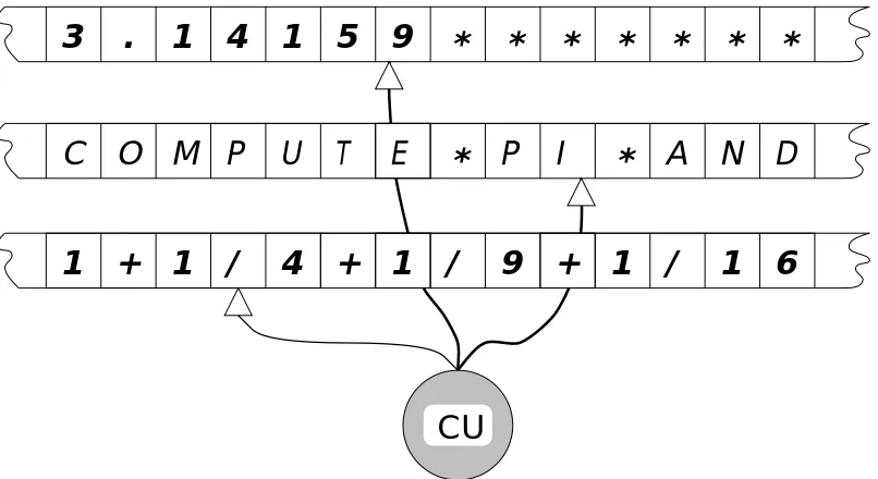
Figure 1.3: A Turing maching with three tapes
1.3.2 Universal Turing machines
Based on the preceding, we can notice a significant difference between Turing machines and real computers: for the computation of each function, we constructed a separate Turing machine, while on real program-controlled computers, it is enough to write an appropriate program. We will now show that Turing machines can also be operated this way: a Turing machine can be constructed on which, using suitable “programs”, everything is computable that is computable on any Turing machine. Such Turing machines are interesting not just because they are more like programable computers but they will also play an important role in many proofs.
Let T = k+ 1,Σ,ΓT, αT, βT, γT and S = k,Σ,ΓS, αS, βS, γS be two Turing machines (k ≥ 1). Let p ∈ Σ∗0. We say that T simulates S with program p if for arbitrary words x1, . . . , xk∈Σ∗0, machineT halts in finitely many steps on input (x1, . . . , xk, p) if and only ifS halts on input (x1, . . . , xk) and if at the time of the stop, the first k tapes of T each have the same content as the tapes ofS.
We say that a (k+ 1)-tape Turing machine is universal (with respect to k-tape Turing machines) if for everyk-tape Turing machineS over Σ, there is a word (program)pwith which T simulates S.
(1.1)Theorem For every numberk≥1and every alphabetΣthere is a(k+ 1)-tape universal Turing machine.
currently in (even if there is only a finite number of states, the fixed machine T must simulate all machines S, so it “cannot keep in its head” the states of S). In each step, on the basis of this, and the symbols read on the other tapes, it looks up in the table the state that S makes the transition into, what it writes on the tapes and what moves the heads make.
First, we give the construction usingk+ 2 tapes. For the sake of simplicity, assume that Σ contains the symbols “0”, “1”, and “–1”. Let S = k,Σ,ΓS, αS, βS, γS be an arbitrary k-tape Turing machine. We identify each element of the state set ΓS\ {STOP} with a word of length r over the alphabet Σ∗0. Let the “code” of a given position of machine S be the following word:
gh1. . . hkαS(g, h1, . . . , hk)βS(g, h1, . . . , hk)γS(g, h1, . . . , hk)
whereg∈ΓS is the given state of the control unit, and h1, . . . , hk∈Σ are the symbols read by each head. We concatenate all such words in arbitrary order and obtain so the word aS. This is what we write on tapek+ 1; while on tapek+ 2, we write a state of machine S, initially the name of the START state.
Further, we construct the Turing machine T which simulates one step or S as follows. On tape k+ 1, it looks up the entry corresponding to the state remembered on tape k+ 2 and the symbols read by the firstkheads, then it reads from there what is to be done: it writes the new state on tape k+ 2, then it lets its first kheads write the appropriate symbol and move in the appropriate direction.
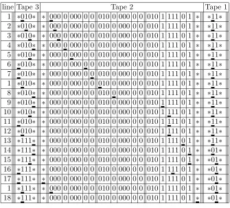
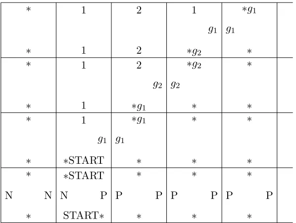
For the sake of completeness, we also define machine T formally, but we also make some concession to simplicity in that we do this only for the case k = 1. Thus, the ma-chine has three heads. Besides the obligatory “START” and “STOP” states, let it also have states NOMATCH-ON, NOMATCH-BACK-1, NOMATCH-BACK-2, MATCH-BACK, WRITE, MOVE and AGAIN. Let h(i) denote the symbol read by the i-th head (1 ≤i ≤3). We describe the functions α, β, γ by the table in Figure 1.4 (wherever we do not specify a new state the control unit stays in the old one).
In the typical run in Figure 1.5, the numbers on the left refer to lines in the above program. The three tapes are separated by triple vertical lines, and the head positions are shown by underscores.
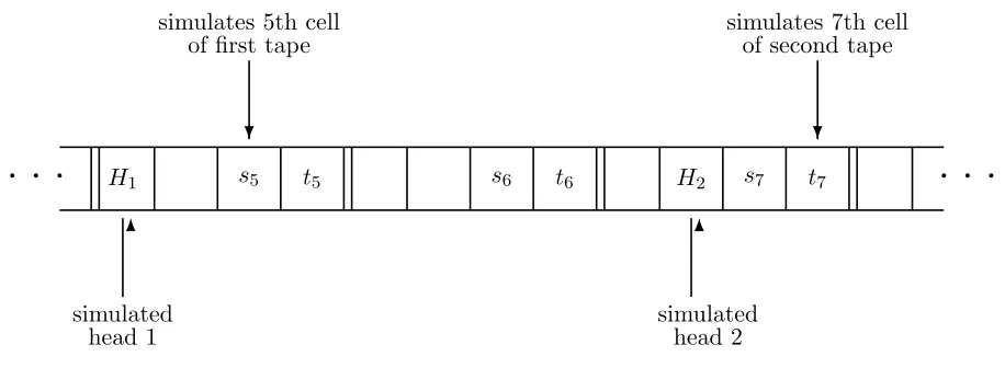
Now return to the proof of Theorem 1.1. We can get rid of the (k+ 2)-nd tape easily: its contents (which is always justrcells) will be placed on cells −1,−2, . . . ,−r. It seems, however, that we still need two heads on this tape: one moves on its positive half, and one on the negative half (they don’t need to cross over). We solve this by doubling each cell: the original symbol stays in its left half, and in its right half there is a 1 if the corresonding head would just be there (the other right half cells stay empty). It is easy to describe how a head must move on this tape in order to be able to simulate the movement of both original heads.
1.9Exercise Write a simulation of a Turing machine with a doubly infinite tape by a Turing machine with a tape that is infinite only in one direction. ♦
START:
1: if h(2) =h(3)=∗ then 2 and 3 moves right;
2: if h(2), h(3)=∗and h(2)=h(3) then “NOMATCH-ON” and 2,3 move right; 8: ifh(3) =∗and h(2)=h(1) then “NOMATCH-BACK-1” and 2 moves right, 3 moves
left;
9: if h(3) =∗and h(2) =h(1) then “MATCH-BACK”, 2 moves right and 3 moves left; 18: ifh(3)=∗ and h(2) =∗then “STOP”;
NOMATCH-ON:
3: if h(3)=∗ then 2 and 3 move right;
4: if h(3) =∗ then “NOMATCH-BACK-1” and 2 moves right, 3 moves left; NOMATCH-BACK-1:
5: if h(3)=∗ then 3 moves left, 2 moves right;
6: if h(3) =∗ then “NOMATCH-BACK-2”, 2 moves right; NOMATCH-BACK-2:
7: “START”, 2 and 3 moves right; MATCH-BACK:
10: ifh(3)=∗ then 3 moves left;
11: ifh(3) =∗ then “WRITE-STATE” and 3 moves right; WRITE:
12: ifh(3)=∗ then 3 writes the symbolh(2) and 2,3 moves right;
13: ifh(3) =∗ then “MOVE”, head 1 writesh(2), 2 moves right and 3 moves left; MOVE:
14: “AGAIN”, head 1 movesh(2); AGAIN:
15: ifh(2)=∗ and h(3)=∗then 2 and 3 move left; 16: ifh(2)=∗ buth(3) =∗then 2 moves left;
17: ifh(2) =h(3) =∗ then “START”, and 2,3 move right.
line Tape 3 Tape 2 Tape 1 1 ∗010∗ ∗ 000 0 000 0 0 010 0 000 0 0 010 1 111 0 1 ∗ ∗11∗ 2 ∗010∗ ∗ 000 0 000 0 0 010 0 000 0 0 010 1 111 0 1 ∗ ∗11∗ 3 ∗010∗ ∗ 000 0 000 0 0 010 0 000 0 0 010 1 111 0 1 ∗ ∗11∗ 4 ∗010∗ ∗ 000 0 000 0 0 010 0 000 0 0 010 1 111 0 1 ∗ ∗11∗ 5 ∗010∗ ∗ 000 0 000 0 0 010 0 000 0 0 010 1 111 0 1 ∗ ∗11∗ 6 ∗010∗ ∗ 000 0 000 0 0 010 0 000 0 0 010 1 111 0 1 ∗ ∗11∗ 7 ∗010∗ ∗ 000 0 000 0 0 010 0 000 0 0 010 1 111 0 1 ∗ ∗11∗ 1 ∗010∗ ∗ 000 0 000 0 0 010 0 000 0 0 010 1 111 0 1 ∗ ∗11∗ 8 ∗010∗ ∗ 000 0 000 0 0 010 0 000 0 0 010 1 111 0 1 ∗ ∗11∗ 9 ∗010∗ ∗ 000 0 000 0 0 010 0 000 0 0 010 1 111 0 1 ∗ ∗11∗ 10 ∗010∗ ∗ 000 0 000 0 0 010 0 000 0 0 010 1 111 0 1 ∗ ∗11∗ 11 ∗010∗ ∗ 000 0 000 0 0 010 0 000 0 0 010 1 111 0 1 ∗ ∗11∗ 12 ∗010∗ ∗ 000 0 000 0 0 010 0 000 0 0 010 1 111 0 1 ∗ ∗11∗ 13 ∗111∗ ∗ 000 0 000 0 0 010 0 000 0 0 010 1 111 0 1 ∗ ∗11∗ 14 ∗111∗ ∗ 000 0 000 0 0 010 0 000 0 0 010 1 111 0 1 ∗ ∗01∗ 15 ∗111∗ ∗ 000 0 000 0 0 010 0 000 0 0 010 1 111 0 1 ∗ ∗01∗ 16 ∗111∗ ∗ 000 0 000 0 0 010 0 000 0 0 010 1 111 0 1 ∗ ∗01∗ 17 ∗111∗ ∗ 000 0 000 0 0 010 0 000 0 0 010 1 111 0 1 ∗ ∗01∗ 1 ∗111∗ ∗ 000 0 000 0 0 010 0 000 0 0 010 1 111 0 1 ∗ ∗01∗ 18 ∗111∗ ∗ 000 0 000 0 0 010 0 000 0 0 010 1 111 0 1 ∗ ∗01∗
q q q H1 s5 t5 s6 t6 H2 s7 t7
6
simulated head 1
?
simulates 5th cell of first tape
6
simulated head 2
?
simulates 7th cell of second tape
[image:17.612.70.528.87.255.2]q q q
Figure 1.6: One tape simulating two tapes
1.11 Exercise Let T and S be two one-tape Turing machines. We say thatT simulates the work of S by program p (here p ∈Σ∗0) if for all wordsx ∈Σ∗0, machine T halts on input p∗x in a finite number of steps if and only if S halts on input x and at halting, we find the same content on the tape ofT as on the tape ofS. Prove that there is a one-tape Turing machine T that can simulate the work of every other one-tape Turing machine in this sense. ♦
1.3.3 More tapes versus one tape
Our next theorem shows that, in some sense, it is not essential, how many tapes a Turing machine has.
(1.2)Theorem For every k-tape Turing machine S there is a one-tape Turing machine T
which replacesS in the following sense: for every wordx∈Σ∗0, machineS halts in finitely many steps on inputx if and only if T halts on inputx, and at halt, the same is written on the last tape ofS as on the tape ofT. Further, if S makes N steps thenT makesO(N2) steps.
Proof We must store the content of the tapes of S on the single tape of T. For this, first we “stretch” the input written on the tape of T: we copy the symbol found on the i-th cell onto the (2ki)-th cell. This can be done as follows: first, starting from the last symbol and stepping right, we copy every symbol right by 2k positions. In the meantime, we write ∗ on positions 1,2, . . . ,2k−1. Then starting from the last symbol, it moves every symbol in the last block of nonblanks 2kpositions to right, etc.
Now we show how T can simulate the steps of S. First of all, T “keeps in its head” which stateS is in. It also knows what is the remainder of the number of the cell modulo 2kscanned by its own head. Starting from right, let the head now make a pass over the whole tape. By the time it reaches the end it knows what are the symbols read by the heads of S at this step. From here, it can compute what will be the new state of S what will its heads write and wich direction they will move. Starting backwards, for each 1 found in an odd cell, it can rewrite correspondingly the cell before it, and can move the 1 by 2k positions to the left or right if needed. (If in the meantime, it would pass beyond the beginning or ending 0, then it would move that also by 2k positions in the appropriate direction.)
When the simulation of the computation of S is finished, the result must still be “com-pressed”: the content of cell 2ki must be copied to cell i. This can be done similarly to the initial “stretching”.
Obviously, the above described machineT will compute the same thing asS. The number of steps is made up of three parts: the times of “stretching”, the simulation and “compression”. Let M be the number of cells on machine T which will ever be scanned by the machine; obviously, M =O(N). The “stretching” and “compression” need timeO(M2). The simulation of one step of S needs O(M) steps, so the simulation needs O(M N) steps. All together, this is still only O(N2) steps.
As we have seen, the simulation of a k-tape Turing machine by a 1-tape Turing machine is not completely satisfactory: the number of steps increases quadratically. This is not just a weakness of the specific construction we have described; there are computational tasks that can be solved on a 2-tape Turing machine in some N steps but any 1-tape Turing machine needs N2 steps to solve them. We describe a simple example of such a task.
A palindrome is a word (say, over the alphabet{0,1}) that does not change when reversed; i.e., x1. . . xn is a palindrome iff xi =xn−i+1 for all i. Let us analyze the task of recognizing a palindrome.
(1.3)Theorem (a) There exists a 2-tape Turing machine that decides whether the input word
x ∈ {0,1}n is a palindrome in O(n) steps. (b) Every one-tape Turing machine that decides whether the input wordx∈ {0,1}n is a palindrome has to makeΩ(n2) steps in the worst case.
Proof Part (a) is easy: for example, we can copy the input on the second tape innsteps, then move the first head to the beginning of the input innfurther steps (leave the second head at the end of the word), and compare x1 withxn,x2 with xn−1, etc., in anothern steps. Altogether, this takes only 3nsteps.
Part (b) is more difficult to prove. Consider any one-tape Turing machine that recognizes palindromes. To be specific, say it ends up with writing a “1” on the starting field of the tape if the input word is a palindrome, and a “0” if it is not. We are going to argue that for every n, on some input of lengthn, the machine will have to make Ω(n2) moves.
Fix any j such that k ≤ j ≤ 2k. Call the dividing line between fields j and j+ 1 of the tape the cutafterj. Let us imagine that we have a little deamon sitting on this, and recording the state of the central unit any time the head passes between these fields. At the end of the computation, we get a sequence g1g2. . . gt of elements of Γ (the length t of the sequence may be different for different inputs), the j-logof the given input. The key to proof is the following observation.
Lemma. Letx =x1. . . xk0. . .0xk. . . x1 and y =y1. . . yk0. . .0yk. . . y1 be two different palin-dromes andk≤j≤2k. Then their j-logs are different.
Proof of the lemma. Suppose that thej-logs ofx andy are the same, sayg1. . . gt. Consider the input z=x1. . . xk0. . .0yk. . . y1. Note that in this input, all the xi are to the left from the cut and all the yi are to the right.
We show that the machine will conclude that zis a palindrome, which is a contradiction. What happens when we start the machine with input z? For a while, the head will move on the fields left from the cut, and hence the computation will proceed exactly as with input x. When the head first reaches field j+ 1, then it is in state g1 by the j-log of x. Next, the head will spend some time to the right from the cut. This part of the computation will be indentical with the corresponding part of the computation with input y: it starts in the same state as the corresponding part of the computation of y does, and reads the same characters from the tape, until the head moves back to field j again. We can follow the computation on input z similarly, and see that the portion of the computation during its m-th stay to the left of the cut is identical with the corresponding portion of the computation with inputx, and the portion of the computation during its m-th stay to the right of the cut is identical with the corresponding portion of the computation with input y. Since the computation with input x ends with writing a “1” on the starting field, the computation with input z ends in the same way. This is a contradiction.
Now we return to the proof of the theorem. For a givenm, the number of different j-logs of length less thanm is at most
1 +|Γ|+|Γ|2+. . .+|Γ|m−1 = |Γ| m−1
|Γ| −1 <2|Γ| m−1.
This is true for any choice of j; hence the number of palindromes whose j-log for some j has length less thanm is at most
2(k+ 1)|Γ|m−1.
There are 2k palindromes of the type considered, and so the number of palindromes for whose j-logs have length at leastm for all j is at least
2k−2(k+ 1)|Γ|m−1. (1.4)
So if we choosemso that this number is positive, then there will be a palindrome for which the j-log has length at least m for all j. This implies that the deamons record at least (k+ 1)m moves, so the computation takes at least (k+ 1)(m+ 1) steps.
1.12 Exercise In the simulation of k-tape machines by one-tape machines given above the finite control of the simulating machine T was somewhat bigger than that of the simulated machineS: moreover, the number of states of the simulating machine depends onk. Prove that this is not necessary: there is a one-tape machine that can simulate arbitrary k-tape machines.
♦
∗(1.13)Exercise Show that everyk-tape Turing machine can be simulated by a two-tape one
in such a way that if on some input, thek-tape machine makes N steps then the two-tape one makes at mostO(NlogN).
[Hint: Rather than moving the simulated heads, move the simulated tapes! (Hennie-Stearns)]
♦
1.14 Exercise Two-dimensional tape.
(a) Define the notion of a Turing machine with a two-dimensional tape.
(b) Show that a tape Turing machine can simulate a Turing machine with a two-dimensional tape. [Hint: Store on tape 1, with each symbol of the two-two-dimensional tape, the coordinates of its original position.]
(c) Estimate the efficiency of the above simulation.
♦
∗(1.15)Exercise Letf : Σ∗
0→Σ∗0 be a function. AnonlineTuring machine contains, besides the usual tapes, two extra tapes. Theinput tapeis readable only in one direction, theoutput tapeis writeable only in one direction. An online Turing machineT computes functionf if in a single run, for eachn, after receivingn symbolsx1, . . . , xn, it writesf(x1. . . xn) on the output tape, terminated by a blank.
Find a problem that can be solved more efficiently on an online Turing machinw with a two-dimensional working tape than with a one-dimensional working tape.
[Hint: On a two-dimensional tape, any one of nbits can be accessed in√nsteps. To exploit this, let the input represent a sequence of operations on a “database”: insertions and queries, and letf be the interpretation of these operations.] ♦
1.16 Exercise Tree tape.
(a) Define the notion of a Turing machine with a tree-like tape.
(b) Show that a two-tape Turing machine can simulate a Turing machine with a tree-like tape. [Hint: Store on tape 1, with each symbol of the two-dimensional tape, an arbitrary number identifying its original position and the numbers identifying its parent and children.]
(c) Estimate the efficiency of the above simulation.
(d) Find a problem which can be solved more efficiently with a tree-like tape than with any finite-dimensional tape.
1.4 The Random Access Machine
Trying to design Turing machines for different tasks, one notices that a Turing machine spends a lot of its time by just sending its read-write heads from one end of the tape to the other. One might design tricks to avoid some of this, but following this line we would drift farther and farther away from real-life computers, which have a “random-access” memory, i.e., which can access any field of their memory in one step. So one would like to modify the way we have equipped Turing machines with memory so that we can reach an arbitrary memory cell in a single step.
Of course, the machine has to know which cell to access, and hence we have to assigne addresses to the cells. We want to retain the feature that the memory is unbounded; hence we allow arbitrary integers as addresses. The address of the cell to access must itself be stored somewhere; therefore, we allow arbitrary integers to be stored in each cell (rather than just a single element of a fintie alphabet, as in the case of Turing machines).
Finally, we make the model more similar to everyday machines by making it programmable (we could also say that we define the analogue of a universal Turing machine). This way we get the notion of aRandom Access Machine or RAM machine.
Now let us be more precise. The memoryof a Random Access Machine is a doubly infinite sequence. . . x[−1], x[0], x[1], . . .of memory registers. Each register can store an arbitrary integer. At any given time, only finitely many of the numbers stored in memory are different from 0.
The program store is a (one-way) infinite sequence of registers called lines. We write here a program of some finite length, in a certain programming language similar to the assembly language of real machines. It is enough, for example, to permit the following statements:
x[i]:=0; x[i]:=x[i]+1; x[i]:=x[i]-1;
x[i]:=x[i]+x[j]; x[i]:=x[i]-x[j];
x[i]:=x[x[j]]; x[x[i]]:=x[j];
IF x[i]≤ 0 THEN GOTO p.
Here, i and j are the addresses of memory registers (i.e. arbitrary integers), p is the address of some program line (i.e. an arbitrary natural number). The instruction before the last one guarantees the possibility of immediate access. With it, the memory behaves as an array in a conventional programming language like Pascal. The exact set of basic instructions is important only to the extent that they should be sufficiently simple to implement, expressive enough to make the desired computations possible, and their number be finite. For example, it would be sufficient to allow the values−1,−2,−3 fori, j. We could also omit the operations of addition and subtraction from among the elementary ones, since a program can be written for them. On the other hand, we could also include multiplication, etc.
The input of the Random Access Machine is a finite sequence of natural numbers written into the memory registers x[0], x[1], . . .. The Random Access Machine carries out an arbitrary finite program. It stops when it arrives at a program line with no instruction in it. Theoutput is defined as the content of the registers x[i] after the program stops.
(1.1)Example [Value assignment] Letiand j be two integers. Then the assignment x[i]:=j
can be realized by the RAM program x[i]:=0
x[i]:=x[i]+1;
...
x[i]:=x[i]+1;
⎫ ⎪ ⎪ ⎬ ⎪ ⎪
⎭ j times
ifj is positive, and x[i]:=0
x[i]:=x[i]-1;
...
x[i]:=x[i]-1;
⎫ ⎪ ⎪ ⎬ ⎪ ⎪ ⎭ |
j| times
ifj is negative. ♦
(1.2)Example [Addition of a constant] Letiand j be two integers. Then the statement x[i]:=x[i]+j
can be realized in the same way as in the previous example, just omitting the first row. ♦ (1.3)Example [Multiple branching] Letp0, p1, . . . , prbe indices of program rows, and suppose that we know that the contents of register isatisfies 0≤x[i]≤r. Then the statement
GOTO px[i]
can be realized by the RAM program IF x[i]≤0 THEN GOTO p0;
x[i]:=x[i]-1:
IF x[i]≤0 THEN GOTO p1;
x[i]:=x[i]-1:
...
IF x[i]≤0 THEN GOTO pr.
(Attention must be paid when including this last program segment in a program, since it changes the content of xi. If we need to preserve the content ofx[i], but have a “scratch” register, say x[−1], then we can do
x[-1]:=x[i];
IF x[-1]≤0 THEN GOTO p0;
x[-1]:=x[-1]-1:
IF x[-1]≤0 THEN GOTO p1;
x[-1]:=x[-1]-1: ...
IF x[-1]≤0 THEN GOTO pr.
Now we show that the RAM and Turing machines can compute essentially the same func-tions, and their running times do not differ too much either. Let us consider (for simplicity) a 1-tape Turing machine, with alphabet {0,1,2}, where (deviating from earlier conventions but more practically here) let 0 stand for the blank space symbol.
Every input x1. . . xnof the Turing machine (which is a 1–2 sequence) can be interpreted as an input of the RAM in two different ways: we can write the numbers n, x1, . . . , xn into the registers x[0], . . . , x[n], or we could assign to the sequencex1. . . xn a single natural number by replacing the 2’s with 0 and prefixing a 1. The output of the Turing machine can be interpreted similarly to the output of the RAM.
We will consider the first interpretation first.
(1.4)Theorem For every (multitape) Turing machine over the alphabet {0,1,2}, one can construct a program on the Random Access Machine with the following properties. It computes for all inputs the same outputs as the Turing machine and if the Turing machine makesN steps then the Random Access Machine makesO(N) steps with numbers ofO(logN) digits.
Proof LetT = 1,{0,1,2},Γ, α, β, γ. Let Γ ={1, . . . , r}, where 1 = START andr = STOP. During the simulation of the computation of the Turing machine, in register 2iof the RAM we will find the same number (0,1 or 2) as in thei-th cell of the Turing machine. Registerx[1] will remember where is the head on the tape, and the state of the control unit will be determined by where we are in the program.
Our program will be composed of parts Qij simulating the action of the Turing machine when in statei and reading symbolj (1≤i≤r−1,0≤j ≤2) and lines Pi that jump toQi,j if the Turing machine is in stateiand reads symbol j. Both are easy to realize. Pi is simply
GOTO Qi,x[1];
for 1≤ i≤i−1; the program part Pr consists of a single empty program line. The program partsQij are only a bit more complicated:
x[x[1]]:= β(i, j); x[1]:=x[1]+2γ(i, j); GOTO Pα(i,j);
The program itself looks as follows. x[1]:=0;
P1 P2
...
Pr Q1,0 ...
Qr−1,2
Turing machine can write anything in at most O(N) registers, so in each step of the Turing machine we work with numbers of lengthO(logN).
Another interpretation of the input of the Turing machine is, as mentioned above, to view the input as a single natural number, and to enter it into the RAM as such. This number a is thus in register x[0]. In this case, what we can do is to compute the digits of a with the help of a simple program, write these (deleting the 1 in the first position) into the registers x[0], . . . , x[n−1], and apply the construction described in Theorem 1.4.
(1.5)Remark In the proof of Theorem 1.4, we did not use the instruction x[i] := x[i] + x[j]; this instruction is needed when computing the digits of the input. Even this could be accomplished without the addition operation if we dropped the restriction on the number of steps. But if we allow arbitrary numbers as inputs to the RAM then, without this instruction the running time the number of steps obtained would be exponential even for very simple problems. Let us e.g. consider the problem that the content aof register x[1] must be added to the content b of register x[0]. This is easy to carry out on the RAM in a bounded number of steps. But if we exclude the instruction x[i] := x[i] +x[j] then the time it needs is at least min{|a|,|b|}. ♦
Let a program be given now for the RAM. We can interpret its input and output each as a word in {0,1,−,#}∗ (denoting all occurring integers in binary, if needed with a sign, and separating them by #). In this sense, the following theorem holds.
(1.6)Theorem For every Random Access Machine program there is a Turing machine com-puting for each input the same output. If the Random Access Machine has running time N
then the Turing machine runs inO(N2) steps.
Proof We will simulate the computation of the RAM by a four-tape Turing machine. We write on the first tape the content of registersx[i] (in binary, and with sign if it is negative). We could represent the content of all registers (representing, say, the content 0 by the symbol “*”). This would cause a problem, however, because of the immediate (“random”) access feature of the RAM. More exactly, the RAM can write even into the register with number 2N using only one step with an integer ofN bits. Of course, then the content of the overwhelming majority of the registers with smaller indices remains 0 during the whole computation; it is not practical to keep the content of these on the tape since then the tape will be very long, and it will take exponential time for the head to walk to the place where it must write. Therefore we will store on the tape of the Turing machine only the content of those registers into which the RAM actually writes. Of course, then we must also record the number of the register in question.
What we will do therefore is that whenever the RAM writes a number yinto a registerx[z], the Turing machine simulates this by writing the string ##y#z to the end of its first tape. (It never rewrites this tape.) If the RAM reads the content of some registerx[z] then on the first tape of the Turing machine, starting from the back, the head looks up the first string of form ##u#z; this valueu shows what was written in the z-th register the last time. If it does not find such a string then it treats x[z] as 0.
“supermachine” in which a set of states corresponds to every program line. These states form a Turing machine which carries out the instruction in question, and then it brings the heads to the end of the first tape (to its last nonempty cell) and to cell 0 of the other tapes. The STOP state of each such Turing machine is identified with the START state of the Turing machine corresponding to the next line. (In case of the conditional jump, if x[i] ≤ 0 holds, the “supermachine” goes into the starting state of the Turing machine corresponding to line p.) The START of the Turing machine corresponding to line 0 will also be the START of the supermachine. Besides this, there will be yet another STOP state: this corresponds to the empty program line.
It is easy to see that the Turing machine thus constructed simulates the work of the RAM step-by-step. It carries out most program lines in a number of steps proportional to the number of digits of the numbers occurring in it, i.e. to the running time of the RAM spent on it. The exception is readout, for wich possibly the whole tape must be searched. Since the length of the tape isN, the total number of steps isO(N2).
1.17 Exercise Write a program for the RAM that for a given positive number a
(a) determines the largest numberm with 2m≤a;
(b) computes its base 2 representation;
♦
1.18 Exercise Let p(x) = a0 +a1x +· · ·+anxn be a polynomial with integer coefficients a0, . . . , an. Write a RAM program computing the coefficients of the polynomial (p(x))2 from those of p(x). Estimate the running time of your program in terms of n and K = max{|a0|, . . . ,|an|}. ♦
1.19 Exercise Prove that if a RAM is not allowed to use the instruction x[i] := x[i] +x[j], then adding the contentaof x[1] to the contentb of x[2] takes at least min{|a|,|b|}steps.
♦
1.20 Exercise Since the RAM is a single machine the problem of universality cannot be stated in exactly the same way as for Turing machines: in some sense, this single RAM is universal. However, the following “self-simulation” property of the RAM comes close. For a RAM program p and inputx, let R(p, x) be the output of the RAM. Let p, x be the input of the RAM that we obtain by writing the symbols ofpone-by-one into registers 1,2,. . ., followed by a symbol # and then by registers containing the original sequence x. Prove that there is a RAM program u such that for all RAM programs pand inputs x we have R(u, p, x) =R(p, x). ♦
head. Arbitrary transformations can be achieved by applying the following three operations repeatedly (and ignoring nodes that become isolated): λ(c, i) := New, where New is a new node; λ(c, i) :=λ(λ(c, j)) and λ(λ(c, i)) := λ(c, j). A machine with this storage structure and these three operations added to the usual Turing machine operations will be called a Pointer Machine.
Let us call RAM’ the RAM from which the operations of addition and subtraction are omitted, only the operationx[i] :=x[i] + 1 is left. Prove that the Pointer Machine is equivalent to RAM’, in the following sense.
For every Pointer Machine there is a RAM’ program computing for each input the same output. If the Pointer Machine has running timeN then the RAM’ runs in O(N) steps.
For every RAM’ program there is a Pointer Machine computing for each input the same output. If the RAM’ has running timeN then the Pointer Machine runs inO(N) steps.
1.5 Boolean functions and Boolean circuits
A Boolean functionis a mapping f :{0,1}n → {0,1}. The values 0,1 are sometimes identified with the values False, True and the variables in f(x1, . . . , xn) are sometimes called Boolean variables, Boolean variables or bits. In many algorithmic problems, there are n input Boolean variables and one output bit. For example: given a graphGwithN nodes, suppose we want to decide whether it has a Hamiltonian cycle. In this case, the graph can be described with N2 Boolean variables: the nodes are numbered from 1 to N and xij (1≤i < j≤N) is 1 if iand j are connected and 0 if they are not. The value of the function f(x12, x13, . . . , xn−1,n) is 1 if there is a Hamilton cycle in G and 0 if there is not. Our problem is the computation of the value of this (implicitly given) Boolean function.
There are only four one-variable Boolean functions: the identically 0, identically 1, the identity and the negation: x→ x= 1−x. We also use the notation¬x. There are 16 Boolean functions with 2 variables (because there are 24 mappings of {0,1}2 into {0,1}). We describe only some of these two-variable Boolean functions: the operation ofconjunction(logical AND):
x∧y =
1 ifx=y= 1, 0 otherwise,
this can also be considered the common, or mod 2 multiplication, the operation of disjunction (logical OR)
x∨y =
0 ifx=y= 0, 1 otherwise,
thebinary addition (logical exclusive OR of XOR) x⊕y=x+ymod 2.
Among Boolean functions with several variables, one has the logical AND, OR and XOR defined in the natural way. A more interesting function is MAJORITY, which is defined as follows:
MAJORITY(x1, . . . , xn) = 1, if at leastn/2 of the variables is 1; 0, otherwise.
These bit-operations are connected by a number of useful identities. All three operations AND, OR and XOR are associative and commutative. There are several distributivity proper-ties:
x∧(y∨z) = (x∧y)∨(x∧z) x∨(y∧z) = (x∨y)∧(x∨z) and
x∧(y⊕z) = (x∧y)⊕(x∧z).
The DeMorgan identities connect negation with conjunction and disjunction: x∧y = x∨y,
x∨y = x∧y.
(1.1)Lemma Every Boolean function is expressible as a Boolean polynomial.
Proof Leta1, . . . , an∈ {0,1}. Let
zi=
xi ifai = 1, xi ifai = 0,
and Ea1,...,an(x1, . . . , xn) =z1∧ · · · ∧zn. Notice thatEa1,...,an(x1, . . . , xn) = 1 holds if and only if (x1, . . . , xn) = (a1, . . . , an). Hence
f(x1, . . . , xn) =
f(a1,...,an)=1
Ea1,...,an(x1, . . . , xn).
The Boolean polynomial constructed in the above proof has a special form. A Boolean polynomial consisting of a single (negated or unnegated) variable is called a literal. We call an elementary conjunctiona Boolean polynomial in which variables and negated variables are joined by the operation “∧”. (As a degenerate case, the constant 1 is also an elementary conjunction, namely the empty one.) A Boolean polynomial is a disjunctive normal form if it consists of elementary conjunctions, joined by the operation “∨”. We allow also the empty disjunction, when the disjunctive normal form has no components. The Boolean function defined by such a normal form is identically 0. In general, let us call a Boolean polynomialsatisfiable if it is not identically 0. As we see, a nontrivial disjunctive normal form is always satisfiable.
By a disjunctive k-normal form, we understand a disjunctive normal form in which every conjunction contains at most kliterals.
(1.2)Example Here is an important example of a Boolean function expressed by disjunctive normal form: the selection function. Borrowing the notation from the programming language C, we define it as
x?y:z=
y ifx= 1, z ifx= 0.
It can be expressed as x?y :z= (x∧y)∨(¬x∧z). It is possible to construct the disjunctive normal form of an arbitrary Boolean function by the repeated application of this example. ♦
Interchanging the role of the operations “∧” and “∨”, we can define theelementary disjunc-tion andconjunctive normal form. The empty conjunction is also allowed, it is the constant 1. In general, let us call a Boolean polynomial a tautologyif it is identically 1.
We found that all Boolean functions can be expressed by a disjunctive normal form. From the disjunctive normal form, we can obtain a conjunctive normal form, applying the distributivity property repeatedly. We have seen that this is a way to decide whether the polynomial is a tautology. Similarly, an algorithm to decide whether a polynomial is satisfiable is to bring it to a disjunctive normal form. Both algorithms can take very long time.
x= 0
y= 1
0
0
QQs
3
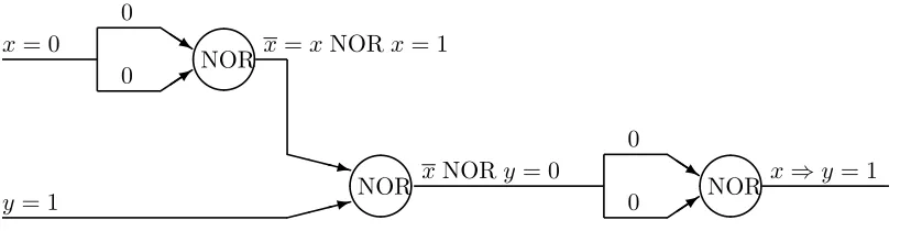
NOR x=xNORx= 1
XXXz
:
NOR xNORy= 0
0 0
3
QQs
[image:29.612.71.480.84.194.2]
NOR x⇒y= 1
Figure 1.7: A NOR circuit computingx⇒y, with assignment on edges
(1.3)Example [Majority Function] Let f(x1, . . . , xn) = 1 if and only if at least half of the variables are 1. ♦
One reason why a computation might be much faster than the size of the Boolean polynomial is that the size of a Boolean polynomial does not reflect the possibility of reusing partial results. This deficiency is corrected by the following more general formalism.
Let G be a directed graph with numbered nodes that does not contain any directed cycle (i.e. isacyclic). The sources, i.e. the nodes without incoming edges, are calledinput nodes. We assign a literal (a variable or its negation) to each input node.
The sinks of the graph, i.e. those of its nodes without outgoing edges, will be called output nodes. (In what follows, we will deal most frequently with circuits that have a single output node.)
To each nodev of the graph that is not a source, i.e. which has some degreed=d+(v)>0, a “gate” is given, i.e. a Boolean function Fv : {0,1}d → {0,1}. The incoming edges of the node are numbered in some increasing order and the variables of the function Fv are made to correspond to them in this order. Such a graph is called acircuit.
Thesizeof the circuit is the number of gates; itsdepthis the maximal length of paths leading from input nodes to output nodes.
Every circuit H determines a Boolean function. We assign to each input node the value of the assigned literal. This is the input assignment, or inputof the computation. From this, we can compute to each nodev a value x(v)∈ {0,1}: if the start nodesu1, . . . , udof the incoming edges have already received a value then v receives the value Fv(x(u1), . . . , x(ud)). The values at the sinks give the output of the computation. We will say about the function defined this way that it iscomputed by the circuit H.
1.22 Exercise Prove that in the above definition, the circuit computes a unique output for every possible input assignment. ♦
If the states of the input lines of the circuit are x and y then the state of the output line is x ⇒ y. The assignment can be computed in 3 stages, since the longest path has 3 edges. See Figure 1.7. ♦
(1.5)Example For a natural number n we can construct a circuit that will simultaneously compute all the functionsEa1,...,an(x1, . . . , xn) (as defined above in the proof of Lemma 1.1) for all values of the vector (a1, . . . , an). This circuit is called the decoder circuit since it has the following behavior: for each input x1, . . . , xn only one output node, namely Ex1,...,xn will be true. If the output nodes are consecutively numbered then we can say that the circuit decodes the binary representation of a number k into the k-th position in the output. This is similar to addressing into a memory and is indeed the way a “random access” memory is addressed. Suppose that a decoder circuit is given for n. To obtain one for n+ 1, we split each output y=Ea1,...,an(x1, . . . , xn) in two, and form the new nodes
Ea1,...,an,1(x1, . . . , xn+1) = y∧xn+1, Ea1,...,an,0(x1, . . . , xn+1) = y∧ ¬xn+1,
using a new copy of the input xn+1 and its negation. ♦
Of course, every Boolean function is computable by a trivial (depth 1) circuit in which a single (possibly very complicated) gate computes the output immediately from the input. The notion of circuits is interesting if we restrict the gates to some simple operations (AND, OR, exclusive OR, implication, negation, etc.). If each gate is a conjunction, disjunction or negation then using the DeMorgan rules, we can push the negations back to the inputs which, as literals, can be negated variables anyway. If all gates are disjunctions or conjunctions then the circuit is called Boolean.
The in-degree of the nodes is is called fan-in. This is often restricted to 2 or to some fixed maximum. Sometimes, bounds are also imposed on the out-degree, orfan-out. This means that a partial