An Efficient Real-time Method of Analysis for Non-coherent Fault
Trees
Rasa Remenyte-Prescott, John D. Andrews
Aeronautical and Automotive Engineering , Loughborough University, Loughborough, UK
Abstract
Fault tree analysis is commonly used to assess the reliability of potentially hazardous industrial systems. The type of logic is usually restricted to AND and OR gates which makes the fault tree structure coherent. In non-coherent structures not only components’ failures but also components’ working states contribute to the failure of the system. The qualitative and quantitative analyses of such fault trees can present additional difficulties when compared to the coherent versions. It is shown that the Binary Decision Diagram (BDD) method can overcome some of the difficulties in the analysis of non-coherent fault trees.
This paper presents the conversion process of non-coherent fault trees to BDDs. A fault tree is converted to a BDD that represents the system structure function (SFBDD). A SFBDD can then be used to quantify the system failure parameters but is not suitable for the qualitative analysis. Established methods, such as the meta-products BDD method, the zero-suppressed BDD (ZBDD) method and the labelled BDD (L-BDD) method, require an additional BDD that contains all prime implicant sets. The process using some of the methods can be time consuming and not very efficient. In addition, in real time applications the conversion process is less important and the requirement is to provide an efficient analysis. Recent uses of the BDD method are for real time system prognosis. In such situations as events happen, or failures occur the prediction of mission success is updated and used in the decision making process. Both qualitative and quantitative assessment are required for the decision making. Under these conditions fast processing and small storage requirements are essential. Fast processing is a feature of the BDD method. It would be advantageous if a single BDD structure could be used for both the qualitative and quantitative analyses. Therefore, a new method, the ternary decision diagram (TDD) method, is presented in this paper, where a fault tree is converted to a TDD that allows both qualitative and quantitative analyses and no additional BDDs are required. The efficiency of the four methods is compared using an example fault tree library.
1. Introduction
Thus, approximation techniques have had to be introduced which resulted in loss of accuracy.
A more convenient form for the logic function from the mathematical viewpoint is that of a Binary Decision Diagram [1]. It overcomes some disadvantages of conventional FTA techniques enabling efficient and exact qualitative and quantitative analyses of both coherent and non-coherent fault trees. The BDD method is efficient for quantifying the system failure likelihood since it does not need the system failure modes as an intermediate step. It is also more accurate as there is no need for the approximations used in the traditional approach of kinetic tree theory [2]. The efficiency and the accuracy of the BDD method is discussed in [3,4].
Rather than analysing the fault tree directly the BDD method first converts the fault tree to a binary decision diagram, which represents the Boolean Equation for the top event. The resulting SFBDD can be used in the quantitative analysis, calculating the top event probability or frequency.
An SFBDD does not provide all the information for the qualitative analysis, since not all the implicant sets of a non-coherent fault tree are necessarily prime and the list may not be complete. This means that it requires more than just a minimisation, as in the coherent case, to produce a full list of prime implicants. The full list can be obtained by applying the consensus theorem [5] to pairs of prime implicant sets involving a normal and negated literal. The first approach to this was presented by Courdet and Madre [6] and further developed by Dutuit and Rauzy [7] where a meta-products BDD is formed. Every basic event is represented by two variables, Px and Sx,
where the first of them represents the relevancy of the component (relevant or irrelevant) and the second variable represents the type of the relevancy (failure relevant or repair relevant). Since a meta-products BDD is in its minimal form, traversing its branches gives all the prime implicant sets.
The second alternative method presented by Rauzy [9] uses the system SFBDD and converts it to the zero-suppressed BDD (ZBDD), presented by Minato [10]. The method requires to label nodes with failed and/or working states of basic events and to decompose prime implicant sets according to the presence of a given state of a basic event. The resulting ZBDD is in its minimal form and traversing its paths from the root vertex to terminal vertex 1 results in all prime implicant sets.
The third alternative method investigated produces a labelled binary decision diagram (L-BDD), presented by Contini in [11] where every basic event is labelled according to its type. The additional information about the occurrence of every basic event is considered at an early stage of the algorithm, i.e. while converting a fault tree to an L-BDD. An L-BDD has two branches, therefore, it does not provide all prime implicant sets. The L-BDD obtained from the fault tree is simplified and then the determination of prime implicant sets is performed where the rules of the calculation depend on the type of a basic event. The L-BDD resulting is minimised.
paper. A TDD has three branches leaving any variable: the 1 branch represents the failure relevance of the component, the 0 branch represents the repair relevance of the component (so far this is a conventional BDD presentation) and the consensus branch represents the irrelevance of the component. A TDD encodes all the prime implicant sets, since while calculating the consensus branch for every node the consensus theorem is applied and all “hidden” prime implicant sets are obtained. However, the TDD can be non-minimal, therefore, the minimisation process needs to be performed removing the non-minimal paths from the 1 and 0 branches. Then the prime implicant sets can be obtained. Also, the obtained TDD can be used for the quantitative analysis as well as the qualitative analysis, therefore, no additional BDDs are required.
The four methods are described in the following sections and demonstrated throughout with the use of an example. Their efficiency is investigated using a library of large example fault trees.
2. Non-coherent fault trees
Fault tree structures can be classified according to their underlying logic. If during fault tree construction the failure logic is restricted to the use of the AND gate and the OR gate, the resulting fault tree is called coherent. If NOT logic is used or directly implied (by for example the use of exclusive OR, XOR, gates) the resulting fault tree can be non-coherent.
Define each component in the system according to an indicator xi to show its status:
working. is component if 0 failed, is component if 1 i i
xi (1)
where i1,2,...,n, n is the number of components in the system.
The fault tree diagram represents a logic structure which can be expressed by a structure function :
working. is system if 0 failed, is system if 1 (2)
=(x), where x = (x1, x2, … , xn).
According to the requirements of coherency [5], a structure function (x) is coherent if:
Each component i must be relevant, i.e. i
i
i,x) (0 ,x)forsomex
1
(
. (3)
(x) is increasing (non-decreasing) for each xi , i.e.
i
i i, ) (0 , )
1
( x x
. (4)
where ) , , , 1 , , , ( ) , 1
( i x1 xi1 xi1 xn
x , (5)
). , , , 0 , , , ( ) , 0
( i x1 xi1 xi1 xn
The second of these conditions means that as the component deteriorates (x fails, so xi
= 1) the system condition either does not change or also deteriorates. If the system is non-coherent for component i then for some state of the remaining components the system is failed then component i works and then when i fails the system is restored to the functioning (non-failed) condition. For example, system failure might occur due to the recovery of a failed component. Alternatively, during system failure, the failure of an additional component may bring the system to a good state. The fault tree is coherent if the NOT logic can be eliminated from the fault tree.
[image:4.595.171.382.217.309.2]
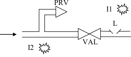
Consider an example of the leak detection system shown in Figure 1.
Figure 1. Leak protection system
A very high pressure gas is flowing as part of a gas transport system. If a leak (L) occurs on the section after the isolation valve (VAL), a gas detection system closes the valve. This stops a build up of the gas concentration in a location where an ignition source (I1) is possible. If the valve works and isolation occurs the high pressure gas can cause a rupture of the pipe and a second leak prior to the isolation valve. There is a permanent ignition source (I2) in this area, therefore, the problem can be avoided by a pressure relief valve (PRV) diverting the gas flow.
An explosion can occur in two ways:
Gas is released prior to isolation valve, when the leak is detected, the isolation valve works but the pressure relief valve fails.
Gas is released after isolation valve, when the leak is detected, the isolation valve fails and the ignition source occurs.
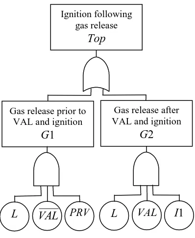
A fault tree representing causes of an ignition following a gas release is shown in Figure 2.
I2
I1
L
Figure 2. Explosion fault tree
Working in a bottom-up way the following logic expression is obtained.
1
I VAL L PRV VAL L
Top , where “+” is OR, “·” is AND.
Therefore,
L,VAL,PRV
and
L,VAL,I1
are prime implicants, as combinations of component conditions (working or failed) which are necessary and sufficient to cause system failure.Also, unlike the reduction of the logic expression for a coherent fault tree the logic Equation for the top event in the non-coherent case does not produce a complete list of all prime implicants. In this example, there is one more failure mode:
} 1 , ,
{L PRV I ,
i.e. if a leak occurs and the pressure relief valve has failed and an ignition source is present on the section after the isolation valve it does not matter if the isolation valve closes or not, an ignition of the gas release will occur.
Therefore, the full logic expression for the Top event is:
1 1 L PRV I I
VAL L PRV VAL L
Top ,
which can be obtained by applying the consensus law:
Y X Y A X A Y A X
A .
There are usually considerably more prime implicant sets than there are minimal cut sets for a coherent representation. Also the prime implicant sets tend to be a larger order (number of elements in a set) than the minimal cut sets. The increase in length of the logic Equation can cause difficulties for large fault trees. A coherent approximation can be obtained by assuming that all working states are TRUE, i.e. the probability of a component working is very close to 1. In the example shown in Figure 2 there are two minimal cut sets,
L,PRV
and
L,VAL,I1
:Ignition following gas release
Top
Gas release prior to VAL and ignition
G1
Gas release after VAL and ignition
G2
. 1 1 1 1 1 I VAL L PRV L I PRV L I VAL L PRV L I PRV L I VAL L PRV VAL L Top
3. Conversion to BDDs
Binary Decision Diagrams can be used for the accurate quantification of fault trees. They do not need to evaluate the prime implicant sets as an intermediate step and do not need approximations. These advantages are critical when analysing non-coherent fault trees and overcome the difficulties encountered with conventional fault tree theory. To utilise the method, the fault tree is converted to a binary decision diagram, representing the structure function SFBDD.
Before the fault tree is converted to a BDD, the fault tree is manipulated so that the NOT logic is “pushed” down the fault tree until it is applied to basic events by using De Morgan’s laws, i.e.
B A B
A , (7)
B A B
A . (8)
Each vertex in a SFBDD has an ite (if-then-else) structure. To illustrate this consider the ite structure ite(x, f1, f0), which means that if x fails then consider function f1, else
consider function f0. Also, f1 lies on the 1 branch of x and f0 lies on the 0 branch.
Constructing the SFBDD from a fault tree initially requires the basic events in the fault tree to be given an ordering. SFBDD construction then moves through the fault tree in a bottom-up manner.
Each basic event is assigned an ite structure
a = ite(a,1,0). (9)
Alternatively, a basic event a is assigned an ite structure:
a= ite(a,0,1). (10)
Dealing with gate inputs:
If J = ite(x,f1, f0) and H = ite(y,g1, g0) represent two inputs to a gate of logic type
then ordering. the in if ) , , ( ordering, the in if ) , , ( 0 0 1 1 0 1 y x g f g f x y x H f H f x H J ite ite (11)
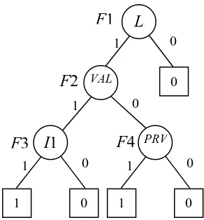
Figure 3. SFBDD for the fault tree in Figure 2
4. Calculation of prime implicant sets
In addition to quantification of the top event, knowledge of prime implicant sets can be valuable in gaining an understanding of the system. It can help to develop a repair schedule for failed components if a system cannot be taken off line for repair. The SFBDD which encodes the structure function cannot be used directly to produce the complete list of prime implicant sets of a non-coherent fault tree.
For example, consider a general component x in a non-coherent system. In a prime implicant a component x can appear in a failed or working state, or can be excluded from the failure mode. In the first two situations x is said to be relevant, in the third case it is irrelevant to the system state. Component x can be either failure relevant (the prime implicant set contains x) or repair relevant (the prime implicant set contains x). A general node in the SFBDD, which represents component x, has two branches. The 1 branch corresponds to the failure of x; therefore, x is either failure relevant or irrelevant. Similarly, the 0 branch corresponds to the functioning of x and so x is either repair relevant or irrelevant. Hence it is impossible to distinguish between the two cases for each branch and the prime implicant sets cannot be identified directly from the BDD.
4.1. Ternary Decision Diagram method
A method to use a ternary decision diagram (TDD) in order to compute the prime implicant sets of a non-coherent fault tree structure is proposed in this section. It employs the consensus theorem and creates, in addition to the two branches of the BDD, a third branch for every node, called the consensus branch. This third branch encodes the “hidden” prime implicant sets. The minimisation algorithm [1] is applied to remove non-minimal paths.
4.1.1. Conversion of fault trees to TDDs
The TDD representation features a node structure with three exit branches. A new ifre
structure is presented which distinguishes not only between relevant and irrelevant components but also it distinguishes between the type of relevancy, i.e. failure relevant and repair relevant. The ifre structure for a node x is given in Figure 4. So if:
1
L
0 0
1
VAL
0
1
1 0
I1
0
PRV
1
1 0
0
F1
F2
= ifre(x, f1, f0, f2), (12)
then
= x f1+xf0 + f2, (13)
where
f2 = f1·f0. (14)
Figure 4. ifre structure
The 1 branch encodes prime implicant sets for which component x is failure relevant, the 0 branch encodes prime implicant sets for which component x is repair relevant, and the “C” branch encodes prime implicant sets for which component x is irrelevant. The ifre structure shown in Figure 4 can be interpreted as follows:
If x is failure relevant then consider f1,
else x is repair relevant then consider f0
else consider f2
endif
Function f2 represents prime implicant sets for which x is irrelevant, i.e. neither failure
nor repair relevant combinations. The “C” branch is not obtained for all components. Therefore, this branch can be kept “empty” for components that are only failure or repair relevant but not both. If the conjunction of the two branches f1·f0 is not required,
f2 = NIL. Symbol NIL identifies cases when the “C” branch is not required and no
Boolean operations that involve this branch are needed. When operating the new symbol in the Boolean algebra, it is defined that NILA= NIL.
The conversion process for computing the TDD from the non-coherent fault tree is an extension to the method used to develop the conventional BDD. Basic events of the fault tree must be ordered. Then the following process is presented:
By the application of De Morgan’s laws push any NOT gates down through the fault tree until it reaches a basic event level.
Each basic event is assigned an ifre structure. If a is only failure or repair relevant:
a= ifre(a,1,0,NIL), (15)
x
f1 f0 f2
1
0
a = ifre(a,0,1,NIL). (16)
If a is failure and repair relevant:
a= ifre(a,1,0,0), (17)
a = ifre(a,0,1,0). (18)
Traversing the fault tree in a bottom-up manner and considering gates whose inputs have been expressed in an ifre format gives:
If J= ifre(x, f1, f0, f2) and H= ifre(y, g1, g0, g2), then
) , , , ( ) , , , ( 0 1 0 1 0 1 0 1 L L L L x K K K K x H J ifre ifre ordering. the in if ordering, the in if y x y x (19)
here K1 f1H,K0 f0H,L1 f1g1,L0 f0g0, K1· K0 – consensus of
K1 and K0, L1· L0 – consensus of L1 and L0.
If component x is failure or repair relevant, K1· K0 = NIL, L1· L0 = NIL in Equation
19.
Within each ifre calculation an additional consensus calculation is performed to ensure all the “hidden” prime implicant sets are encoded in the TDD. It calculates the product of the 1 and the 0 branch of every node and thus identifies the consensus of each node.
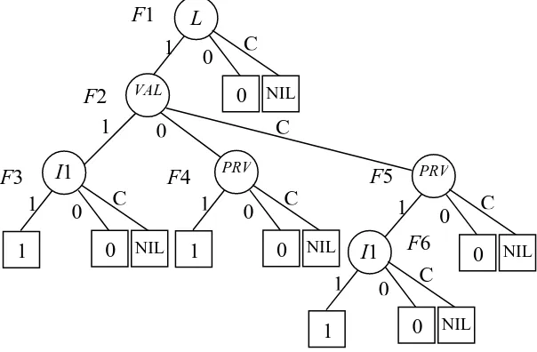
[image:9.595.150.452.440.638.2]Consider the fault tree in Figure 2. Introducing the ordering of basic events L < VAL < PRV < I1 and applying the rules described in Equations (15)-(19) gives the TDD in Figure 5.
Figure 5. The TDD for the fault tree shown in Figure 2
It can be seen that the TDD in Figure 5 is different from the SFBDD in Figure 3 only with its “C” branch that represents the intersection of the 1 and 0 branches. Only for node F2 a new structure F5 is created. The other nodes have the “C” branch leading to value NIL, since they encode variables that only appear as failure or repair relevant To obtain prime implicant sets non-minimal combinations from every path need to be removed. 1 L 1 VAL 0 C F1 F2 0 0 C NIL 1 1 I1 F3 0 0 C NIL PRV 1 1 F4 0 0 C NIL 1 PRV 1 1 I1 F5 F6 0 0 C
NIL
0
0 C
4.1.2. Minimisation of TDDs
Once the TDD has been computed there is no guarantee that the resulting structure will be minimal, i.e. produce the prime implicant sets exactly. In order to perform the qualitative analysis a minimisation procedure needs to be implemented.
The algorithm developed by Rauzy for minimising the BDD [1] can be extended to create a minimal consensus TDD that encodes only the prime implicant sets.
Consider a general node in the TDD which is represented by the function F, where
F = ifre(x, G, H, K). (20)
Since there are three types of variables in the TDD (failure relevant, repair relevant and both), the minimisation process is described for these three cases.
Minimal solutions of G, H and K are denoted as Gmin, Hmin and Kmin. Let δ be a
minimal solution of G, which is not a minimal solution of K. Then the intersection of δ and x ( x) will be a minimal solution of F. Similarly, let γ be a minimal solution
of H, which is not a minimal solution of K, and the intersection of γ and x ( x) will be a minimal solution of F.
Case 1 - x is failure relevant only
In Equation (20) K = NIL and the calculation of prime implicant sets is equivalent to the BDD case where the “C” branch does not exist, i.e.
solmin(F) =(x)Hmin. (21) The set solmin(F) represents the minimal solutions of F by removing any minimal
solutions of G that are also minimal solutions of H.
Case 2 - x is repair relevant only
Again, in Equation (20) K = NIL and the calculation of prime implicant sets is defined as:
solmin(F) =( x)Gmin. (22) The set solmin(F) represents the minimal solutions of F by removing any minimal
solutions of H that are also minimal solutions of G.
Case 3 - x is failure and repair relevant
The set of all the minimal solutions of F is given as:
solmin(F) =( x)( x)Kmin. (23) The set solmin(F) represents the minimal solutions of F by removing any minimal
solutions of G and H that are also minimal solutions of K.
4.1.3. Obtaining prime implicant sets from TDDs
Case 1
Traversing the 1 branch of node x results in a failed state of a component in a particular failure mode. Traversing the 0 branch of node x does not include that component in a particular failure mode.
Case 2
Traversing the 0 branch of node x results in a repaired state of a component in a particular failure mode. Traversing the 1 branch of node x does not include that component in a particular failure mode.
Case 3
Traversing the 1 branch of node x results in a failed state of a component in a particular failure mode. Traversing the 0 branch of node x results in a working state of a component in a particular failure mode. Finally, traversing the “C” branch of node x does not include that component in a particular failure mode at all
Traversing the TDD in Figure 5 from the root vertex to terminal vertices 1 gives three prime implicant sets.
F1-F2-F3 {L, VAL, I1} F1-F2-F4 {L,VAL,PRV}
F1-F2-F5-F6 {L, PRV, I1}
The TDD method provides a good alternative technique for performing the qualitative analysis for non-coherent fault trees.
4.2. Established methods
This section presents the existing methods for converting non-coherent fault trees to BDDs and obtaining prime implicant sets. In the later section the efficiency of all methods, including the TDD method, will be investigated and compared using some example fault trees.
4.2.1. Meta-products BDD method
This method converts a SFBDD to a meta-products BDD which produces all prime implicant sets. A meta-products BDD obtained is in its minimal form.
4.2.1.1.Conversion of SFBDDs to meta-products BDDs
An alternative notation was developed in [6,7] that associates two variables with every component x. The first variable, Px, denotes relevancy and the second variable,
Sx, denotes the type of relevancy, i.e. failure or repair relevant. A meta-product,
. to belongs nor
neither if
, ,
) (
x x P
x if S P
x if S P
MP
x x x
x x
(24)
The proposed algorithm by Dutuit and Rauzy [7] is used for calculating the meta-products BDD of a fault tree from the BDD. The meta-meta-products BDD is always minimal, therefore it encodes the prime implicant sets exactly.
In order to present the algorithm, consider node F in a SFBDD, where F = ite(x, F1, F0). The meta-products BDD, that describes prime implicant sets using Equation (24), is expressed as:
PI(F) = ite(Px, ite(Sx, P1, P0), P2), (25)
where
P2 = PI(F1·F0), (26)
P1 = PI(F1) · 2P , (27)
P0 = PI(F0) ·P2. (28)
x is the first element in the variable ordering, PI(F) represents the structure of a meta-products BDD, PI is used to denote the prime implicants.
P2 encodes the prime implicants for which x is irrelevant, P1 encodes the prime implicants for which x is failure relevant and P0 encodes the prime implicants for which x is repair relevant.
If not all the basic events in the variable ordering appear on the particular path, then
PI(F) = ite(
j x
P , 0, PI(F)). (29)
here xjis before xi and xj does not appear on the current path from the root node to
node F.
If F is a terminal node, then
PI(0) = 0, (30)
PI(1) = ite(
i x
P , 0, ite( 1
i
x
P , 0,…, ite(
n x
P , 0, 1))). (31)
where xi, …, xnare basic events from the variable ordering that have not yet been
considered in the process.
Each node in Figure 3 is considered in turn. Applying Equations (25)-(28) to node F1 gives:
PI(F1) = ite(PL, ite(SL, PI(F2) · 1, PI(0) · 1), PI(F2 · 0)) = ite(PL, ite(SL, PI(F2), 0), 0).
Now consider node F2. Applying Equation (25) to node F2 gives:
PI(F2) = ite(PVAL, ite(SVAL, PI(F3)·PI
F3 · F4
, PI(F4)·PI
F3 · F4
), PI(F3 · F4)).First of all, PI(F3 · F4) is calculated using Equations (25)-(28):
Applying Equations (29)-(31) gives the two following expressions: PI(F3) = ite(PPRV, 0, ite(PI1, ite(SI1, 1, 0), 0)),
PI(F4) = ite(PPRV, ite(SPRV, ite(PI1, 0, 1), 0), 0).
Negation PI
F3 · F4
is calculated swapping terminal vertices 1 and 0.
F3 · F4
PI = ite(PPRV, ite(SPRV, ite(PI1, ite(SI1, 0, 1), 1), 1), 1).
Since there are no repeated parts between PI(F3) and PI
F3 · F4
,PI(F3)·PI
F3 · F4
= PI(F3).The same simplification is applied to PI(F4) and PI
F3 · F4
,PI(F4)·PI
F3 · F4
= PI(F4).The resulting meta-products BDD for the BDD in Figure 3 is shown in Figure 6.
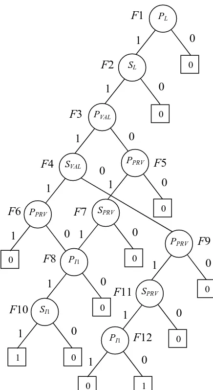
4.2.1.2.Obtaining prime implicant sets
Now it is possible to obtain the meta-products and identify the prime implicant sets. Every path from the root node to a terminal 1 gives a prime implicant set.
L VAL VAL PRV I1 I1
L S P S P P S
P {L, VAL, I1}
L VAL VAL PRV PRV I1
L S P S P S P
P {L,VAL,PRV}
L VAL PRV PRV I1 I1
L S P P S P S
P {L, PRV, I1}
For example, in the first meta-product PLsignifies that component L is relevant and SL
signifies that component L is failure relevant. The same with components VAL and I1.
PRV
P means that component PRV is irrelevant. Hence the prime implicant set obtained is {L, VAL, I1}.
Figure 6. Meta-products BDD for calculating prime implicant sets
4.2.2. ZBDD method
An alternative method presented by Rauzy in [9] uses the idea of zero-suppressed BDDs (ZBDD) introduced by Minato in [10]. The method requires to label nodes with failed and/or working states of basic events and to decompose prime implicant sets according to the presence of a given state of a basic event.
4.2.2.1.Zero-Suppressed BDDs
Zero-suppressed BDDs are BDDs based on a reduction rule. This data structure provides a unique and compact representation which is more efficient and simpler than the usual BDDs when manipulating sets in combinatorial problems. The following reduction rules for BDDs are applied:
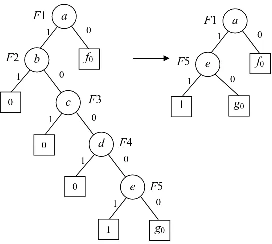
Eliminate all the nodes that have the 1 branch pointing to terminal vertex 0. Then connect the branch that was pointing to the eliminated node to the BDD structure beneath the 0 branch of the eliminated node as shown in Figure 7.
Share all equivalent BDD structures as for original BDDs. 1
1 0
0 PL
0
SL 0
1 0
PVAL
1 SVAL
0
1 0
0
PI1
1
1 0
SI1
0 1
0
PPRV
0
1 0
0
PPRV
1
0
SPRV
0
1 0
0
PPRV
1
0
SPRV
0
1
0 1
PI1
0 F1
F2
F3
F4 F5
F6 F7
F8
F9
F10
F11
Figure 7. Elimination process
ZBDDs automatically suppress basic events that do not appear in prime implicant sets. It is very efficient when calculating sets with basic events that are far apart in the variable ordering scheme. For example, in Figure 7 the left-hand BDD contains a prime implicant set {a, e}. The established variable ordering is a<b<c<d<e. The ZBDD obtained by applying the reduction rules brings basic events close since the intermediate nodes (F2, F3, F4) can be eliminated.
4.2.2.2.Decomposition rule
The principle of this algorithm is to traverse the SFBDD that encodes structure function = ite(x, f1, f0) in a depth-first way and to build a ZBDD that encodes the
prime implicant sets of in a bottom-up way.
The rule is divided in four cases:
Case 1: if basic event x appears in its failed and working states then
PI() = xS1xS0S2, (32) where
S2 = PI( f1∙ f0 ), (33)
S1 = PI( f1 ) \ S2, (34)
S0 = PI( f0 ) \ S2. (35)
Here “\” is operator without [1] that is used minimising conventional BDDs.
Case 2: if basic event x appears in its failed state only then
PI() = xS1S0, (36)
where
S0 = PI( f0 ), (37)
1
a
f0
0
1
b
0
F1
0
F2
c
0 1
F3
0
1
d
0
0 e
0 1
1 g0
F4
F5
1
a
f0
0
1
e
0
F1
1 F5
S1 = PI( f1 ) \ S0. (38)
Case 3: if basic event x appears in its working state only then it is considered in a similar way to case 2.
Case 4: if basic event x does not appear in the system then
PI() = PI( f1 + f0 ). (39)
The resulting ZBDDs retain the variable ordering from the SFBDD. In addition, working states of basic events that appear in both states are incorporated in the ordering scheme, i.e. they appear after the basic event in its failed state in the ordering scheme.
4.2.2.3.ZBDD Example
Consider the SFBDD in Figure 3. Introduce the variable ordering for the ZBDD method L < VAL < VAL < PVR < I1. Applying the rules described in Equations (32)-(39) gives the ZBDD in Figure 8.
Each node is considered in the bottom-up way.
F3 = ite(I1, 1, 0), PI(F3) = ite(I1, 1, 0) - Both vertices are terminal. F4 = ite(PRV, 1, 0), PI(F4) = ite(PRV, 1, 0) - Both vertices are terminal.
F2 = ite(VAL, F3, F4), PI(F2) = ite(VAL, S1, ite(VAL, S0, S2)) - Basic event VAL
appears in both failed and working states. Here, following Equations (33)-(35) gives:
S2 = PI( F2∙F3 ) = PI(ite(PRV, ite(I1, 1, 0), 0)) = ite(PRV, ite(I1, 1, 0), 0) - Both basic
events PRV and I1 appear only in their failed state.
S1 = PI(F3) \ S2 = ite(I1, 1, 0) - There are no repeated paths in F3that are covered by
S2.
S0 = PI(F4) \ S2 = ite(PRV, 1, 0) - There are no repeated paths in F4that are covered
by S2.
Therefore,
PI(F2) = ite(VAL, ite(I1, 1, 0), ite(VAL,ite(PRV, 1, 0), ite(PRV, ite(I1, 1, 0), 0))). According to Equation (36)
F1 = ite(L, F2, 0), PI(F1) = ite(L, PI(F2), 0) - Basic event L appears only in its failed state.
After the last substitution we obtain:
PI(F1) = ite(L, ite(VAL, ite(I1, 1, 0), ite(VAL, ite(PRV, 1, 0),
ite(PRV, ite(I1, 1, 0), 0))), 0).
Figure 8. The ZBDD for the SFBDD in Figure 3
Every path from the root vertex to terminal vertex 1 presents a prime implicant set. Therefore, this ZBDD contains three prime implicant sets:
F1-F2-F3 {L, VAL, I1} F1-F2-F4-F5 {L,VAL,PRV}
F1-F2-F4-F6-F7 {L, PRV, I1}
The ZBDD is an efficient technique where all prime implicant sets are described by a compact and easy handling structure.
4.2.3. Labelled variable method
The labelled variable method [11] provides another alternative method for constructing BDDs for non-coherent fault trees. BDDs constructed using this conversion approach consist of variables that are labelled according to their type. They are called labelled binary decision diagrams (L-BDDs).
The background for this method is that the current analysis algorithms consider the fault tree structure as a Boolean function in which all variables have the same properties, whereas the operations to be applied to determine the prime implicant sets are dependent on the variables’ type. For example, variables that appear in their failure and success states can appear in combinations of events which lead to system failure in both states, and which are not covered by the SFBDD obtained. In the L-BDD method it is convenient to consider this additional information about the type of a variable during the conversion process itself. The aim of the L-BDD method is to construct and analyse a L-BDD in which all variables are labelled with their type.
F3
F2 F1
F6
1
L
0 0
1
VAL
0
1
1 0
I1
0
0 1
VAL
VAL 0
1
1 0
PRV
0 1
PRV
0
1
1 0
I1
0
F4
F5
4.2.3.1.Conversion of fault trees to L-BDDs
The structure function (x) of a non-coherent fault tree may contain three different types of basic events. For example, the function (x)abacbc contains a double form (DF) variable a that appears in both states, a single form positive (SFP) variable b and a single form negative (SFN) variable c. In the further presentation the SFP variable x will be simply presented by x, the SFN variable x will be labelled as “$x” and the DF variable x will be labelled as “&x”.
The conversion process for computing the L-BDD from the non-coherent fault tree is an extension to the method used to develop the SFBDD. Basic events of the fault tree must be ordered. Then the following process is performed:
By the application of De Morgan’s laws push any NOT gates down through the fault tree until it reaches a basic event level.
Each basic event is assigned an ite structure as in Equation (9) or Equation (10).
Traversing the fault tree in a bottom-up manner and considering gates whose inputs have been expressed in an ite format using Equation (11).
The last rule Equation (11) of this algorithm is extended presenting some additional rules that incorporate labelled variables.
Considering the ordering &x < x < $x implements the following Equations: If J = ite(x,f1, f0) and H = ite($x,g1, g0),
then J H ite(&x,f1g0, f0g1) (40) If J = ite(&x,f1, f0) and H = ite(x,g1, g0),
thenJH ite(&x,f1g1, f0g0) (41) If J = ite(&x,f1, f0) and H = ite($x,g1,g0),
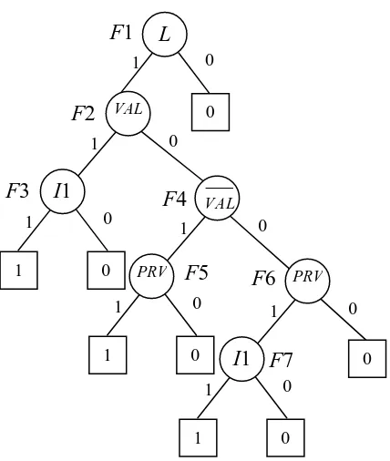
thenJH ite(&x,f1g0,f0g1) (42) Applying the conversion rules given in Equations (9)-(11) and Equations (40)-(42) to the fault tree in Figure 2 results in a L-BDD presented in Figure 9. The variable ordering is L < VAL < PRV < I1.
Figure 9. BDD with labelled variables for the fault tree in Figure 2
1
L
0 0
1
&VAL
0
I1
1
1 0
0
PRV
1
1 0
0
F1
F2
The resulting L-BDD is equivalent to its SFBDD in Figure 3, if DF variable “&VAL” is replaced by variable VAL. The L-BDD does not provide all the information for the qualitative analysis, therefore some additional calculations are performed in order to get all prime implicant sets.
4.2.3.2.Simplification of L-BDD
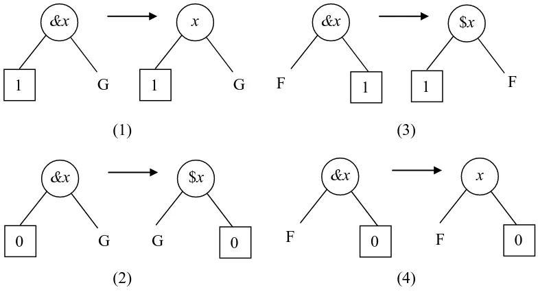
[image:19.595.96.488.249.462.2]The most complex rules of the qualitative analysis of the L-BDD are applied to nodes with DF variables. Therefore, it is convenient to reduce the number of DF variables before calculating prime implicant sets. The rules are applied on the parts of the L-BDD that have a terminal vertex. Simplification rules are shown in Figure 10.
Figure 10. Simplification rules for the L-BDD
The example L-BDD in Figure 9 is in its simplest form, therefore the simplification rules are not applied.
4.2.3.3.Obtaining prime implicant sets from L-BDD
Let structure function be:
0
1 x f
f xi i
(43)
where the two residues are:
) ,..., 1 ,..., ( 1
1 x xn
f (44)
) ,..., 0 ,..., ( 1
0 x xn
f (45)
Let PI() be the prime implicants of . Visiting the L-BDD in the bottom-up way the procedure to be applied to the node xi to determine the prime implicants is as
follows:
If xi has label “&” then
2 0
1 $
)
( x S x S S
PI i i (46)
where &x
1 G
x
1 G
&x
0 G
$x
0 G
&x
1 F
$x
1 F
&x
0 F
x
0 F
(1)
(2)
(3)
2 0 0 2 1 1 0 1
2 f f ,S f \S ,S f \S
S . (47)
Else
0 1
)
( S f
PI (48)
where
0 1
1 \
,
$x S f f
or
xi i
(49)
“\” is the operator “without” proposed by Rauzy [1]. Some extra rules are applied in the cases with labelled variables.
For example, f1\ f0 gives the L-BDD of f1 in which the combinations of f1 repeated
in f0 are removed.
The heaviest operation is the intersection S2 = f1 f0 that, however, is applied only
when dealing with “&” type variables. It calculates the “hidden” prime implicant sets. If there are no “&” type variables, the L-BDD contains all prime implicant sets.
The rules for writing the prime implicant sets from an L-BDD are straightforward. On the path from the root to any terminal node:
For variables x, “$x” do not consider the negated part,
For variables “&x” consider the right branch as x.
Consider the L-BDD shown in Figure 9. Prime implicant sets can be calculated using Equations (46)-(49).
Since the variable of node F2 is a DF variable, i.e. it appears in the fault tree in both success and failure states, the intersection of its 1 and 0 branches is calculated in order to get all prime implicant sets. This process is similar to the calculation of the “C” branch in the TDD method.
P = F3 · F4 = ite(I1, 1 , 0) · ite(PRV, 1 , 0) = ite(PRV, ite(I1, 1 , 0), 0), PI(P) = PRV · S1 + f0, here S1 = I1, f0 = 0,
PI(P) = PRV · I1.
Since there are no repeated paths between the 1 branch and the structure P and none between the 0 branch and the structure P, prime implicant sets of F2 are as follows:
PI(F2) = VAL · I1 + VAL · PRV + PRV · I1. Finally, the last node F1 is considered:
PI(F1) = L · S1 + f0, here S1 = PI(F2), f0 = 0,
PI(F1) = L · (VAL · I1 + VAL · PRV + PRV · I1). The three prime implicant sets are obtained:
{L, VAL, I1}, {L,VAL,PRV}, {L, PRV, I1}.
5. Quantitative analysis of non-coherent
5.1.Quantification of a non-coherent system using the TDD
In order to perform the quantitative analysis for non-coherent fault trees using the BDD method, a non-coherent fault tree is converted to a SFBDD that represents the structure function of the fault tree. In the TDD method the non-coherent fault tree is converted to the TDD that has three branches from each node. The third branch is created to encode all prime implicants of the system. However, the TDD can be used not only for the qualitative analysis but also for the quantitative analysis.
Consider node F in the TDD, F = ifre(x, f1, f0, f1f0). The structure function (x) was
expressed in (13), i.e. (x) xf1xf0 f1f0. Using the pivotal decomposition to the structure function of order n it is possible to express it in terms of structure functions that are of order n-1. Pivoting (x) about variable x and applying the absorption law to Equation 35 gives:
1 1 0
0 1 0
1 0) , 0 ( ) , 1 ( )
(x x i x x i x x f f f x f f f xf xf
. (50)
Then the expectation of (x) is obtained and the top event probability is calculated:
q Q(f1)
1 q
Q(f0) EQSYS x x x . (51)
Therefore, the probability of the top event, QSYS, is the sum of the probabilities of the
disjoint paths through the TDD. The disjoint paths, that are taken into account, can be found by tracing all paths from the root vertex via the 1 and 0 branches to terminal 1 vertices. The disjoint paths via the “C” branch are not included in the quantification process.
If the quantitative analysis is required as well as the qualitative analysis, the TDD before the minimisation can be used for the quantification process. Additional calculations for obtaining the SFBDD are not required.
5.2.Quantitative analysis using other methods
Consider a node F in the SFBDD, F = ite(x, f1, f0). The structure function (x) is
expressed as (x)xf1 xf0, which is adequate to the expression in (50). Therefore, the probability of the top event, QSYS, is obtained as a sum of probabilities of the
disjoint paths through the SFBDD. Quantitative analysis is performed in this way applying the meta-products BDD method and the ZBDD method, where the SFBDD is obtained after fault tree conversion prior to the qualitative analysis.
In the L-BDD method the quantitative analysis is adequate, i.e. the probability of the top event, QSYS, is the sum of the probabilities of the disjoint paths through the
L-BDD. In this case each variable &x is treated as x, and $x – as x.
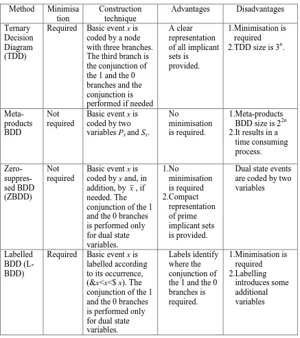
6. Comparison of the four methods
Method Minimisa tion
Construction technique
Advantages Disadvantages
Ternary Decision Diagram (TDD)
Required Basic event x is coded by a node with three branches. The third branch is the conjunction of the 1 and the 0 branches and the conjunction is performed if needed
A clear representation of all implicant sets is
provided.
1.Minimisation is required
2.TDD size is 3n.
Meta-products BDD
Not required
Basic event x is coded by two variables Px and Sx.
No
minimisation is required.
1.Meta-products BDD size is 22n 2.It results in a
time consuming process. Zero- suppres-sed BDD (ZBDD) Not required
Basic event x is coded by x and, in addition, by x, if needed. The
conjunction of the 1 and the 0 branches is performed only for dual state variables. 1.No minimisation is required 2.Compact representation of prime implicant sets is provided.
Dual state events are coded by two variables
Labelled BDD (L-BDD)
Required Basic event x is labelled according to its occurrence, (&x<x<$ x). The conjunction of the 1 and the 0 branches is performed only for dual state variables.
[image:22.595.81.518.80.573.2]Labels identify where the conjunction of the 1 and the 0 branches is required. 1.Minimisation is required 2.Labelling introduces some additional variables
Table 1. Comparison of the four techniques
Table 1 gives a short overview of all four construction techniques. It highlights the main advantages and disadvantages of the four approaches. The TDD method provides a clear and efficient representation of prime implicant sets when the “C” branch for a node is created if needed. Also, using the ZBDD a compact representation of prime implicant sets is obtained which does not require the minimisation process. The least favourable technique is the meta-products BDD method where two variables are assigned for every basic event. Due to this feature the size of the BDD and the processing time is increased unavoidably.
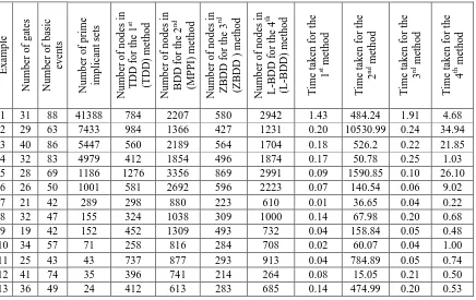
performance over 13 example fault trees was obtained, since each method may perform well on some fault trees dependent upon the fault tree structure. The complexity of the 13 fault trees is indicated in columns 2, 3 and 4 of Table 2, representing the number of gates, the number of events and the number of prime implicant sets in their solution.
The number of nodes using the TDD method, the meta-products BDD method, the ZBDD method and the L-BDD method are presented in columns 5, 6, 7 and 8 respectively. The number of nodes in the TDD method describes the sum of the number of nodes in the TDD before the minimisation and the number of nodes in the TDD after the minimisation. The number of nodes for the second method covers the number of nodes in the SFBDD and the meta-products BDD. For the ZBDD method the number of nodes in the SFBDD and the number of nodes in the ZBDD is given. The number of nodes in the L-BDD method contains the sum of the number of nodes in the L-BDD before applying the minimisation and the number of nodes in the minimised L-BDD.
Similarly, the processing time in seconds covers the time taken to convert example fault trees to BDDs and perform the qualitative analysis. Results of processing time are shown in columns 9, 10, 11 and 12 of Table 2 for the four methods respectively.
E x am p le Nu m b er o f g ates Nu m b er o f b asic ev en ts Nu m b er o f p rim e im p lican t sets Nu m b er o f n o d es in T DD fo r th e 1 st (T DD) m eth o d Nu m b er o f n o d es in B DD fo r th e 2 nd (MPPI ) m eth o d Nu m b er o f n o d es in Z B DD fo r th e 3 rd (Z B DD ) m eth o d Nu m b er o f n o d es in L -B DD fo r th e 4 th (L -B DD) m eth o d T im e tak en f o r th e 1
st m
eth o d T im e tak en f o r th e 2
nd m
eth o d Ti m e tak en f o r th e 3
rd m
eth o d T im e tak en f o r th e 4
th m
eth
o
d
1 31 88 41388 784 2207 580 2942 1.43 484.24 1.91 4.68
2 29 63 7433 984 1366 427 1231 0.20 10530.99 0.24 34.94
3 40 86 5447 560 2189 564 1704 0.18 526.2 0.22 21.85
4 32 83 4979 412 1854 496 1874 0.17 50.78 0.25 1.03
5 28 69 1186 1276 3356 869 2991 0.09 1590.85 0.10 26.10
6 26 50 1001 581 2692 596 2223 0.07 140.54 0.06 9.02
7 21 42 289 298 880 223 610 0.01 36.65 0.04 0.22
8 32 47 155 324 1038 309 1000 0.14 67.98 0.20 0.68
9 19 42 152 452 1309 493 732 0.04 158.84 0.05 0.48
10 34 57 71 258 816 284 708 0.02 60.07 0.04 1.00
11 25 43 43 737 877 293 913 0.04 784.89 0.05 0.74
12 41 74 35 396 741 214 264 0.08 15.05 0.21 0.50
[image:23.595.84.520.360.635.2]13 36 49 24 412 613 283 685 0.14 474.99 0.20 0.53
Table 2. Calculation results for example fault trees
could be decreased using any other method instead of the conventional meta-products BDD method.
The TDD method performed as well as the ZBDD method. Both methods were more efficient than the meta-products BDD method and the L-BDD method in terms of the number of nodes and the processing time. For all example fault trees the TDD method was faster than the ZBDD method. This is due to the efficient representation of prime implicant sets in the TDD method, when the third branch is created if needed. According to the number of nodes, for some examples the ZBDD method was better than the TDD method. This outcome is explained by a compact representation of prime implicant sets in the ZBDD method and no requirement of additional storage for a minimal BDD.
The second worst result was obtained using the L-BDD method. The weaknesses of the L-BDD method are the introduction of the three different types of basic events and the requirement for minimisation before obtaining prime implicant sets.
Overall, these results show that the TDD method is an efficient method to obtain prime implicant sets, when all prime implicant sets are obtained by performing the conjunction of the two branches of each node. Information about the failure and/or repair relevancy of the component is used to identify if the conjunction of the two branches is needed, which makes the process efficient. Finally, the same TDD that is used to represent prime implicant sets before the minimisation can be used for the quantitative analysis, no additional structure is required.
7. Discussion of Real-time BDD Analysis
Recent research into autonomous vehicles (such as UAVs) is using BDDs to calculate the probability of mission failure at the current point in time. At a point in time certain phases may be known to have completed successfully (i.e. NOT failed, therefore requiring a non-coherent analysis), component failures may exist (as indicated by a fault detection and identification tool) or other events may have occurred. By establishing the potential causes of mission failure (prime implicant sets) and the updated likelihood decisions are made regarding the future operation of the autonomous vehicle.
The fault tree to BDD conversion in this application is done off-line and so conversion time is important but not critical. Storing and processing the BDD on-board of the vehicle are the factors which are the more critical in determining which is the best method to use.
Since the Ternary Decision Diagram permits one representation for both qualitative and quantitative analyses and has a very good efficiency compared to the alternatives this representation is advantageous in this particular circumstance.
8. Conclusions
method can be used as an alternative way for qualitative and quantitative analyses of non-coherent fault trees. This paper proposes a new alternative technique that produces a ternary decision diagram, which allows to calculate all prime implicants directly. Established methods - the conventional algorithm that produces a meta-products BDD, the zero-suppressed BDD method and the labelled BDD method are presented and their efficiency is compared using some example fault trees. Efficiency analysis indicates that the new proposed TDD method is the fastest method and it provides an efficient representation of prime implicant sets. Another advantage of the TDD method is that it is suitable for both qualitative and quantitative analyses of non-coherent fault trees, whereas in the existing techniques two separate BDDs need to be constructed if the full analysis is required.
9. References
1. Rauzy, A. New Algorithms for Fault Tree Analysis, Reliability Engineering and System Safety, 40, pp203-211 (1993)
2. Vesely, W.E. A Time Dependent Methodology for Fault Tree Evaluation, Nuclear Design and Engineering, 13, pp337-360, (1970)
3. Sinnamon, R.M. and Andrews, J.D. Improved efficiency in qualitative fault tree analysis, Quality and Reliability Engineering International, 13, pp293-298 (1997) 4. Sinnamon, R.M. and Andrews, J.D. Improved accuracy in quantitative fault tree
analysis, Quality and Reliability Engineering International, 13, pp285-292 (1997) 5. Andrews, J.D. To Not or Not to Not!!, Proceedings of the 18th International
System Safety Conference, pp267-274 (2000)
6. Courdet, O. and Madre, J.-C. A New Method to Compute Prime and Essential Prime Implicants of Boolean Functions, Advanced Research in VLSI and Parallel Systems, pp113-128 (1992)
7. Dutuit, Y. and Rauzy, A. Exact and Truncated Computations of Prime Implicants of Coherent and Non-Coherent Fault Trees with Aralia, Reliability Engineering and System Safety, 58, pp225-235 (1997)
8. Sasao, T. Ternary Decision Diagrams and their Applications, Chapter 12, pp269-292, Representations of Discrete Functions, Edited by Sasao, T. and Fujita, M. Kluwer Academic Publishers (1996)
9. Rauzy, A. Mathematical Foundation of Minimal Cutsets, IEEE Transactions on Reliability, volume 50, 4, pp389-396 (2001)
10.Minato, S. Zero-Suppressed BDDs for Set Manipulation in Combinatorial Problems, Proceedings of the 30th ACM/IEEE Design Automation Conference, DAC’93, pp272-277 (1993)
11.Contini, S. Binary Decision Diagrams with Labelled Variables for Non-Coherent Fault Tree Analysis, (European Commission, Joint Research Centre) 2005
12.Bartlett, L.M. and Andrews, J.D. Comparison of Two New Approaches to Variable Ordering for Binary Decision Diagrams, Quality and Reliability Engineering International, 17, pp151-158 (2001)