The Problem of Scheduling in Parallel Machines:
A Case Study
F. Charrua Santos and Pedro M. Vilarinho
Abstract — In this paper, a problem of scheduling tasks in uniform parallel machines with sequence-dependent setup times is presented. The problem under analysis contains a particular set of constraints, including equipment capacity, task precedences, lot sizing and task delivery plan.
The complexity of the mathematical programming model developed for this problem hasn’t permitted to find one solution using optimising methods and so the authors have developed a heuristic based on the simulated annealing algorithm which allows obtaining nearly-optimal solutions. Index Terms—Schedulling parallel machine, uniform parallel machine, simulated annealing, sequence dependent setup times.
I. INTRODUCTION
The scheduling problem for uniform parallel machines with sequence dependent setup times should be considered as an operational planning problem, occurring in different types of industries, namely in the textile industry.
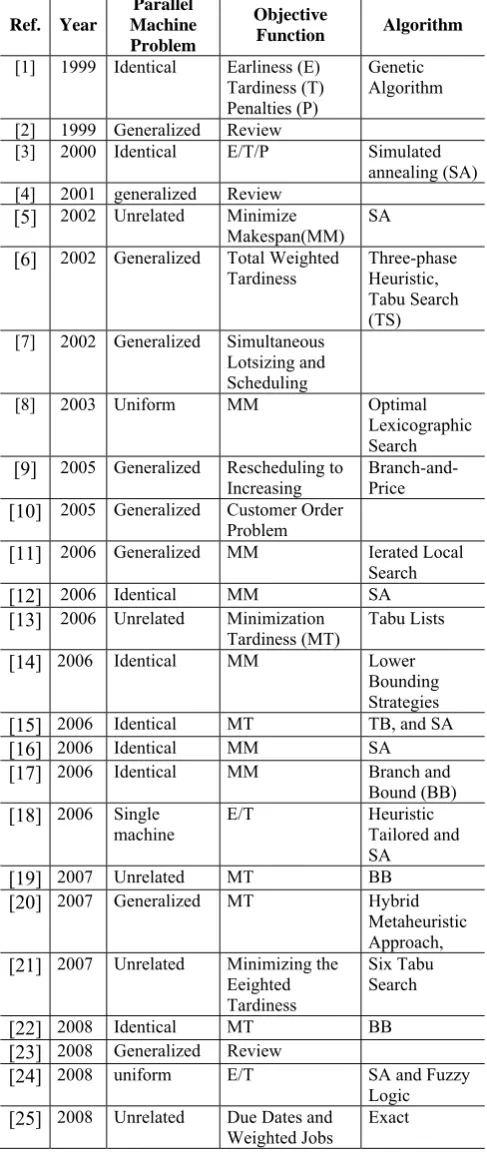
In the first part of this work, the problem under analysis is defined, comparing it with other types of scheduling problems referred in literature and focusing the aspects that make them unique (see Table I).
The mathematical programming model developed by the authors for the problem of scheduling in uniform parallel machines with sequence dependent setup times will be later presented, defining the proposed objective function and the constraints for the problem.
The complexity of the studied model doesn’t permit to find the optimal solution. To solve this, the authors used the simulated annealing algorithm to obtain “nearly-optimal” solutions for the problem.
This heuristic has been incorporated in a tool to support decision makers and some computational results will later be presented to show the good performance reached by using such heuristic.
This work contributes to the exisitng litterature by presenting a new tool to solve a problem that occurrs in real industrial environments. This is the reason why a textile industry example was chosen to inspire the present work.
The results obtained through the application of this particular heuristic show the importance of using a structured approach in scheduling the production, in
F. Charrua Santos is with the Department of Electromechanical Engineering, University of Beira Interior, Calçada Fonte do Lameiro, Covilhã, Portugal, phone: +351 275 329 754; fax: +351 275 329 972, e-mail: [email protected] ;
[image:1.595.301.545.201.782.2]Pedro M. Vilarinho is with the Department of Economics, Management and Industrial Engineering, University of Aveiro, Campo Universitário de
Table I – Problems referred in literature
Ref. Year
Parallel Machine Problem
Objective
Function Algorithm [1] 1999 Identical Earliness (E)
Tardiness (T) Penalties (P)
Genetic Algorithm
[2] 1999 Generalized Review
[3] 2000 Identical E/T/P Simulated
annealing (SA) [4] 2001 generalized Review
[5] 2002 Unrelated Minimize
Makespan(MM) SA [6] 2002 Generalized Total Weighted
Tardiness
Three-phase Heuristic, Tabu Search (TS) [7] 2002 Generalized Simultaneous
Lotsizing and Scheduling
[8] 2003 Uniform MM Optimal
Lexicographic Search [9] 2005 Generalized Rescheduling to
Increasing Branch-and-Price [10] 2005 Generalized Customer Order
Problem
[11] 2006 Generalized MM Ierated Local
Search
[12] 2006 Identical MM SA
[13] 2006 Unrelated Minimization Tardiness (MT)
Tabu Lists
[14] 2006 Identical MM Lower
Bounding Strategies [15] 2006 Identical MT TB, and SA
[16] 2006 Identical MM SA
[17] 2006 Identical MM Branch and
Bound (BB) [18] 2006 Single
machine
E/T Heuristic Tailored and
SA
[19] 2007 Unrelated MT BB
[20] 2007 Generalized MT Hybrid
Metaheuristic Approach, [21] 2007 Unrelated Minimizing the
Eeighted Tardiness
Six Tabu Search
[22] 2008 Identical MT BB
[23] 2008 Generalized Review
comparison with the results obtained in a reference plant where mainly “ad hoc” actions were normally taken.
II. CHARACTERIZATION OF THE PROBLEM The scheduling production problem has largely been analysed by the scientific community and these particular problems are frequently joined together according to the industrial environment characteristics found in each particular site.
In this work the classification used by Allahverdi et al. [1] will be used, subdividing the scheduling problems as follows: Single machine; Parallel machines; Flow Shop Job shop; Open shop.
The problem of scheduling parallel machines was studied by Mokotoff, (2001) [18]. In this review paper, this type of problems is presented according to the following criteria: Identical parallel machines; Uniform parallel machines and Unrelated parallel machines
Generally is accepted that in some types of industrial environments, particularly in the processes industry, sequencing is relevant, but on the other hand other researchers say the opposite stating that the optimization efforts are systematically denied by the reality found in each plant and enterprise
In the following sections of this work, this is supported by the experience acquired in fabrics producers and its main purpose is to evaluate how important the scheduling problem is to the productive process efficiency in this particular case of industrial environment.
The study has allowed identifying a production lot sizing and scheduling problem associated with the planning stage in the weaving area of fabrics manufacturing.
According to the adopted classification referred above, the problem now being analysed fits entirely in the type of lot sizing and scheduling in uniform parallel machines with setup times and costs sequence dependent, width restrictions and tardiness penalties.
According to the search made in the specialized available literature, a lot of situations concerning identical parallel machines with setup times and sequence dependent [18], have been found, but none of them considers the lot sizing and scheduling restrictions associated neither with the equipments nor to tardiness penalties. As a result of such situation, is well worth to make a more detailed analysis in the search of the best solution for such drawback.
It is now important to refer the problem concerning types of setups associated to scheduling; the problem deals with job sequences, material pieces, weaving equipments and looms. Equal material pieces, being sequenced in the same machine, are joined in batches, so the setup time between equal pieces, i.e., for pieces belonging to the same batch, is zero.
Nevertheless, when the amount of equal pieces reaches a certain established value, the batch limit, a setup should then take place. The batch limit varies according to the type of piece of material. We can now conclude, (this is one point that diverges from what has been found in literature), that for equal pieces, having a continuous sequence in the same machine, two preparation times can take place: a) it will be zero, if the limit dimension has not been reached; b)
it will have a certain value (the set-up time) if any other situation occurs.
III. PROBLEM STATEMENT AND FORMULATION The generalized version of the problem can be described in the same way as when occurs a problem of tasks sequence in parallel uniform machines, having different delivery times and setups variable times between tasks, and also depending on their sequence in the queue.
The problem under analysis has the following characteristics:
1) the throughput is stable along the time 2) the demand is known in the planning horizon. 3) the overall production can adequately be represented by a limited set of pieces (p=1, …, P)
4) production is made in a set of machines joined together according to their characteristics in G groups of machines (g=1, … G) each one having NMg machines
5) to each piece p is associated a delivery date dp. 6) any piece delivered after the established delivery date, implies a certain penalty, expressed by a factor ρ for each previously established time unit of delay.
7) each piece is processed in one only machine of a defined group.
8) each piece p can be processed in machines belonging to any group which has the required characteristics for the processing, considering tppg the processing time of the piece p in one of the machines belonging to the group g (p=1, …, P and g=1, …, G).
9) the setup time of each machine that processes the piece j after having produced the piece i is know and represented by sij and is independent of the machine in which the piece has been processed , but always associated to the characteristics of the sequence of the pieces .
10) the setup time of the machine that produces the piece i in the beginning of the queue is known and represented by s0i
11) Lamax represents the maximum amount of pieces than can be joined and processed together continuously without any setup operation being required.
12) Each piece has its own assembly and colour and when pieces that are processed continuously in the same machine have the same assembly and colour there is no need for a setup operation. The amount of different assembly combinations is A, and Na (a=1,…,A) is the set of pieces having the same assembly and colour (having a as reference)
13) M is an large positive number
14)
otherwise 0
g group the in processed
be can i piece the if 1
ig
Before providing a mathematical formulation, the following variables have be defined:
cp date of conclusion of the piece p tp tardiness of the piece p
otherwise 0 g group of k machine in j by followed is i task if 1 xijkg otherwise 0 0 group the of k machine to assigned is i if 1 yikg otherwise 0 g group the of k machine same the in processed are j and i tasks the 1 zij
The problem can then be modelled as one of mixed integer programming:
k g ijg akg i i A 1 a ; Na j , i
i k g i j k g
' ij ijkg ig ikg t . . s . x p . y min
R
s
(1)G 1,..., = g ; M 1,..., = k , 1 x g
j 0jkg
(2) G ,..., 1 g ; M ,..., 1 k ; P ,..., 1 j p s ) x 1 .( M c g jg jg 0 jkg 0 j (3)
j
i ;
i ijkg jkg g
G ,..., 1 g ; M ,..., 1 k ; P ,..., 1 j , y x (4)
j
i
;j ijkg jkg g
G ,..., 1 g ; M ,..., 1 k ; P ,..., 1 i , y x (5) G ,..., 1 g ; M ,..., 1 k ; P ,..., 1 j ,i p s c ) x 1 .( M c g jg ' ij i ijkg j (6) P ,...., 1 i , t d
ci i i (7)
k g ikg ikg
P ,..., 1 i , 1 * y (8) G ,..., 1 g ; M ,..., 1 k ; P ,..., 1 j ,i , z 1 y
yikg jkg ij (9)
A ,..., 1 a ; N , z . s
sij' ij ij i,j a
(10) A ,..., 1 a ; N , R x a j , i akg max a Na j , i ijkg
L
(11)In the objective function,
1) is the total production time and is the sum of the following four items: i) delay time; ii) setup time between different pieces; iii) setup time between equal pieces; iv) processing time.
• the delay time is given by the sum of all the delays occurred during the planning horizon, multiplied by a penalty factor.
• the setup time is given by the sum of all the setup times during the planning horizon.
• the processing time is given by the sum of all the pieces processing times included in the planning analysis.
The model constraints can be interpreted as follows: 2) constraints ensuring that only one initial preparation can take place in each machine k belonging to group g
3) constraints ensuring that the conclusion time of piece j, when processed in the beginning of the queue of machine k, belonging to group g, is equal to the initial setup time of piece j plus the processing time of piece j in the machine g. 4) constraints ensuring that if the setup time for piece j takes place in one k machine belonging to group g, then j is either preceded by another piece, or from the initialposition and so will be processed in machine k of group g.
5) constraints ensuring that if the preparation for piece j occurs in one machine k of group g, then j either is preceded from another piece or is situated in the last position and so will be processed in machine k of group g.
4 e 5) both restrictions together ensure that pieces P will be processed by the k machines of g groups, which means that all the pieces will be processed. At the same time, these simultaneous conditions guaranty that each machine only processes one piece at a time, considering that the number of setups plus the initial preparation gives the total number of processed pieces.
6) constraints ensuring that the processing of each piece once started cannot be interrupted.
7) constraints ensuring that the delay time of piece i is given by the difference between the conclusion date and the delivery date.
From the general conditions of the problem can be concluded that ti is a positive number and so delay only happens when ci is larger than di.
8) constraints ensuring that each piece is manufactured only once and in a compatible machine
9) constraints ensuring that if one piece i is processed in the machine k belonging to group g, and another piece j is processed in the machine k of the same group g, then both pieces are processed in the same machine.
10) constraints ensuring that the preparation time taken by changing from piece i to piece j in group g is zero if i and j have the same type of assembly and colour, assuming a known value Sijg if the previous conditions are not carried out.
11) constraints ensuring that when the number of equal pieces, continuously sequenced, exceeds the maximum batch dimension, then, the resulting setups are taken in account.
IV. SIMULATED ANNEALING ALGORITHM The simulated annealing (SA) is a no deterministic search local technique used when trying to find solutions in combinatory optimization problems, based on the analogy of the minimum state energy of a physical system compared to the minimum cost in a combinatory optimization problem [26], [27]
Simulated annealing is an extension of the local search algorithm, based on a possible initial solution. For that initial solution is attached a certain cost, Zx, and from that initial solution on is reached a neighbouring solution with a cost represented by Zy. The difference between Zy and Zx is represented by ΔZyx.
If the opposite happens, solution Zx will be maintained. This procedure will keep being repeated till new improvements stop emerging, what means that a local minimum was attained. The local search algorithms are very easy to apply, but, as can be understood, they may converge to a unique local minimum, what implies that significant deviations from the optimal solution can take place.
The simulated annealing turns up in order to improve the performance of this type of algorithm once it permits to overtake one local minimum with a certain probability, i.e, it is possible to accept one solution having a certain probability when ΔZyx=Zy-Zx>0. In the SA the probability of the solution to be accepted is determined by the accepting function given by the expression exp(-Z/T), where T is the control parameter which, by analogy, is equivalent to the factor temperature in the controlled metals cooling process. A random number is generated from a uniform distribution (0, 1) and compared with the value of the accepting function, if not it won’t be accepted.
This function has the following effect: minor increases in the value of the accepting function have less probability to be accepted, once the larger the value of the temperature is, the bigger is the probability of an increase of the accepting function to be accepted. While the temperature is decreasing, less is the probability of a worst solution to be accepted. [27].
V. THE DEVELOPED HEURISTIC
In order to solve the optimization problem through the SA algorithm, the algorithm parameters have to be established [28], [29], namely:
• the initial and final values of the temperature which are the control parameters.
• the dimension of each temperature level, ie, the number of iterations made for each value of the temperature. In the case being analysed the number of iterations in each level was considered proportional to the problem dimension and is given by 2N, where N represents the number of batches to be scheduled.
• temperature tuning.
The utilization of the SA still requires the determination of: Initial solution; Neighbouring solutions; Cost function
A. Description of the Heuristic for the determination of the initial solution
This heuristic role for the purpose above mentioned is limited to respect the restrictions of the problem, namely in the particular problem studied by the authors, the compatibility between the width of the task to be performed and the required equipments involved. Starting from the task of bigger width, it selects all the compatible equipments and distributes the task to the less charged equipment.
the initial solution will have the following characteristics:
• the tasks having equal characteristics,; assembly and colour for the same delivery date are joined in batches.
• Each machine has a waiting rank where a certain number of batches having the same known processing time are included.
• The batches have a preparation time depending on the process sequence in the processing machine.
• There is a “Z” cost expressed by units of time for the obtained sequencing, being this value the result of adding up the processing time, the preparation times and the time penalty when such is applicable.
• The transport unit is the batch.
As a result of the application of this heuristic, a possible solution is obtained and, then, from that point on, close solutions will be generated.
B. Heuristic for the determination of neighbouring solutions
Neighbouring solutions are obtained through random batch transferences and swaps. A neighbour solution can be generated by two ways
• Random transference with width restriction The random transference when width restriction takes place consists in moving one random batch, positioned in the same queue, to other queue, only taking in account the width restriction.
• Random swaps with width restriction
In this case, random batches either belonging to the same queue, or in other ranks where only width restrictions exist, are chosen.
A comprehensive heurist, as happens in our case, only based on random transfers or swaps, leads to a wider search space, which can take more time to converge to a minimum local.
In the present work, the above random criteria has been adopted, having been considered to be more important for the particular problem being analysed, in first place the quality of the solution and not the time involved for the execution.
C. Heuristic description for the cost “Z” evaluation
As explained before, the initial solution is a scheduling of grouped batches per machine, which implies that the system will be prepared to evaluate the time associated for the processing. In this case, the system, queue by queue, or, in other words, machine by machine, will evaluate the sum of the processing times associated to each batch.
After being done the exchange or transference, the system, queue after queue, will calculate the number of preparations of each existing type and proceed to the total calculation for all the preparations.
Considering all the times involved in production, the one where more calculation difficulties are met is the delay time calculated period by period. The system should consider the possibility of any advance or delay in a machine for a certain period of time is transferred to the following period. Such evaluation requires an additional computational effort, especially when big dimensions problems are faced.
Cost “Z” is then the result of adding up processing and setup times plus the penalties caused by eventually failed delivery dates.
VI. COMPUTATIONAL RESULTS
A good solution is the one resulting from the ratio production capacity versus processing and setups requirements.
If the processing time plus the setup time requirements exceeds the capacity, the lower limit should take in account a penalty time for the tardiness.
The penalty factor can take the form of a parameter. Considering the amplitude of the problem that we are dealing with, is not an easy job to find an algorithm for computing the lower limit, covering with success all the situations.
An algorithm presenting good performances in environments where many groups of machines, many machines per group and many periods of time are involved was chosen; the authors think that is best adjusted algorithm to the practical case that they were dealing with.
A. Description of the carried out tests
Tests were made having in mind the structure of the identified problem. Ten scenarios having increasing complexity were created, the last one corresponding to the practical case being analyzed. For each of the sceneries, a significant number of tests have been done using different parameters.
Generally speaking, the characteristics of the tests that have been done are shown in Table II.
In Table III is described the information contained in each column of TableII.
Scenario 10 concerns the practical studied case consisting on scheduling 5828 tasks distributed by 232 batches. These batches are distributed by 48 machines. The machines are grouped in 4 different categories according to its own characteristics. The planning horizon is on this case 10 weeks.
A certain amount of processing operation was made for the different sceneries in order to appreciate the best obtained performance. For this purpose the value δ has been changed in the range between 0, 0001 to 0, 1.
In each of the scenerios, four values for δ were tested, and for each value a significant number of processing operations.
Table IV shows the obtained results. In this table, Zm represents the best obtained performance, Z0 represents the initial solution. LB represents the lower band obtained
TableII – Peformed tests
Table III – Description of table II
through the applied heuristic, ((Zm-LB)/LB)*100 the percentage of improvement of the solution related to the lower band, and ((Z0-Zm)/Zm)*100 the percentage of improvement of the solution related to the initial solution.
The analysis of the results let us conclude that the algorithm performance is greatly related to the structure and dimension of the problem. This was an expected fact, once the evaluation criteria, (convergence to the lower band), was developed, having as reference the experience of the skilled planner in big dimension problems.
[image:5.595.318.550.73.298.2]In fact the lower band reflects the value hat would be considered by the planner as the best for a problem having such size. In the analysed industrial environments, and this
Table IV – Obtained results
Scenrio Zm Z0 LB
1 12790 12790 12790
2 37910 49995 28040
3 79027 164908 65819
4 50739 50739 50739
5 62160 66910 57640
6 55345 74071 46495
7 61550 73585 58025
8 70445 80925 61950
9 248494 318428 231411
10 2053181 2273021 1946458
Scenrio ((Zm-LB)/LB)*100 ((Z0-Zm)/Zm)*100
1 0,00 0,00
2 35,20 31,88
3 20,07 108,67
4 0,00 0,00
5 7,84 7,64
6 19,03 33,84
7 6,07 19,55
8 13,71 14,88
9 7,38 28,14
Sce. Mach. Gr.
Mach. Nº
Nº Per.
Nº Ass. Col.
Nº Task
Nº batch
1 1 1 3 1 3 50 3
2 1 1 3 2 3 105 9 3 1 1 5 2 5 292 20 4 2 2 3 2 6 189 6 5 2 2 3 2 6 235 12 6 2 2 4 4 10 242 32 7 2 4 2 4 7 295 13 8 4 4 2 4 7 295 13 9 4 8 4 6 14 1148 50 10 4 48 10 39 87 5828 232
Column Description
Sce. Identifies the constructed scenario
Mach. Gr. Indicates the number of groups considered in the scenario Mach. Nº Indicates the total number of machines
considered in the scenario
Nº Per. Indicates the number of periods, the number of different delivery dates in the planning horizon. Within the same period all the tasks have the same delivery date.
Nº Ass. Number of different assemblies considered in the scenario
Col. Number of different colours
considered in the scenario. Nº Task Indicates the number of tasks
fact should be underlined, the used methodology for dimensioning an sequencing of the batches is very close to the heuristic applied to generate the initial solution of the presented work.
VII.CONCLUSIONS
According to what has been said, considering the type of industry studied, the obtained results show a clear importance of the scheduling problem, when defining strategies for the planning of the production
As can be understood, it is not possible to extend the obtained results to every other type of industrial environment. Nevertheless, the now described study permits thinking in promising results in other different industrial environments.
The authors tried to demonstrate on this study, that, when well dominating the skilled tasks of planning and processing, it is possible to find something between the more conceptual approaches and the ones where more mathematics is involved, This will certainly induce to the development of new instruments, although with some expected limitations, can provide an important tool in what concerns one of the most vital managing information.
REFERENCES
[1] Sivrikaya-Serifoglu, F. e G. Ulusoy, “Parallel machine scheduling with earliness and tardiness penalties”, Computers and Operations Research, Vol. 26,1999, pp. 773–787.
[2] Allahverdi, Gupta e Aldowaisan, "A review of scheduling research involving setup considerations", International. Journal. Management Science, Vol. 27, 1999, pp 219-239,
[3] Radhakrishnan e Ventura, "Simulated annealing for parallel machine scheduling with earliness tardiness penalties and sequence-dependent set-up times", International Journal of Production Research., Vol. 38, Nº. 10, 2000, pp.2233- 2252.
[4] Mokotoff, "Parallel Machine scheduling problems: A survey", Ásia-Pacific Journal of Operational Research, Vol.18, 2001, pp.193-242. [5] Anagnostopoulos e Rabadi, “A simulated annealing algorithm for the
unrelated parallel machine scheduling problem”, Robotics, Automation and Control and Manufacturing: Trends, Principles and Allpications, pp15-120, 2002.
[6] Eom, D.H., H.J. Shin, I.H. Kwun, J.K Shim, e S.S. Kim “Scheduling jobs on parallel machines with sequence-dependent family set-up times”, International Journal of Advanced Manufacturing Technology, Vol. 19, 2002, pp. 926–932.
[7] 7Meyr, “Simultaneous lotsizing and scheduling on parallel machines”, European Journal of Operational Research, Vol.139, 2002, pp.277–292.
[8] Liao e Lin, “Makespan minimization for two uniform parallel machines”, International Journal of Production Economics, Vol. 84, 2003, pp. 205-213.
[9] Curry e Peters, “Rescheduling parallel machines with stepwise increasing tardiness and machine assignment stability objectives”, International Journal of Production Research, Vol. 43,2005, pp. 3231-3246.
[10]Jaehwan e Marc, Scheduling Parallel Machines for the Customer Order Problem, Journal of Scheduling, Vol. 8, 2005, pp. 49-74. [11]Tang e Luo, “A new ILS algorithm for parallel machine scheduling
problems”, Journal of Intelligent Manufacturing, Vol. 17, 2006, pp. 609-619.
[12] Wen-Chiunge, Chin-Chia e Chen "A simulated annealing approach to makespan minimization on identical parallel machines" The International Journal of Advanced Manufacturing Technology, Vol. 31, Nº 3-4, 2006, pp. 328-334.
[13]Chen, J.F., “Minimization of maximum tardiness on unrelated parallel machines with process restrictions and setups”, The International Journal of Advanced Manufacturing Technology, 29, 2006, pp. 557-563.
[14]Haouari, Gharbi e Jemmali, “Tight bounds for the identical parallel machine scheduling problem”, International Transactions in Operational Research, Vol. 13, 2006, pp. 529-548.
[15]Kim, S.I., H.S. Choi e D.H. Lee, “Scheduling algorithms for parallel machines with sequence-dependent set-up and distinct ready times: minimizing total tardiness”, Proceedings of the Institution of Mechanical Engineers Part B-Journal of Engineering Manufacture´, Vol. 221, 2007, pp. 1087-1096.
[16]Lee, Wu e Chen, “A simulated annealing approach to makespan minimization on identical parallel machines”, International Journal of Advanced Manufacturing Technology, Vol. 31, 2006, pp. 328-334. [17]Nessah, Yalaoui e Chu, “A branch and bound algorithm to minimize
total weighted completion time on identical parallel machines with job release dates”, Proceedings of International Conference on Service Systems and Service Management, Vol. 2, 2006, pp. 1192-1198.
[18]Rabadi, Moraga e Al-Salem, “Heuristics for the Unrelated Parallel Machine Scheduling Problem with Setup Times”, Journal of Intelligent Manufacturing, Vol. 17, 2006, pp. 85-97.
[19]Shim e Kim, “Minimizing total tardiness in an unrelated parallel-machine scheduling problem”, Journal of the Operational Research Society, Vol. 58, 2007, pp. 346-354.
[20]Anghinolfi D e M. Paolucci, “Parallel machine total tardiness scheduling with a new hybrid metaheuristic approach”, Computers and Operations Research, Vol. 3, 2007, pp. 3471-3490.
[21]Logendran, R., B. McDonell e B Smucker, “Scheduling unrelated parallel machines with sequence-dependent setups”, Computers & Operations Research, Vol. 34, 2007, pp. 3420-3438.
[22]Oh e Kim, “A branch and bound algorithm for an identical parallel machine scheduling problem with a job splitting property”, Computers & Operations Research, Vol. 35, 2008, pp. 863-875. [23]Allahverdi, Ng, Cheng, Mikhail e Kovalyov, “A survey of cheduling
problems with setup times or costs”, European Journal of Operational Research, Vol. 187, 2008, pp. 985–1032.
[24]Raja, K., V. Selladurai, R. Saravanan e C. Arumugam, “Earliness-tardiness scheduling on uniform parallel machines using simulated annealing and fuzzy logic”, Proceeding of the Institution of Mechanical Engineers part B-Journal of Engineering Manufacture´, Vol. 222, 2008, pp. 333-346.
[25]Rocha P. L., M. G. Ravetti e G. R. Mateus, “Exact algorithms for a scheduling problem with unrelated parallel machines and sequence and machine-dependent setup times”, Computers and Industrial Engineering, Vol. 35, 2008, pp. 1250-1264.
[26]Metropolis, Rosenbluth, e Teller” Equation of state calculations by fast computing machine”, Journal of Chemical Physics, Vol.21, 1953, pp.1087-1092.
[27]Kirkpatrick, Gelatt e Vecchi “Optimization by_Simulated Annealing”, Science, Vol.220, 1983, pp.671-680.
[28]Madhavan, K., Weighted earliness-tardiness minimization for jobs with sequence dependent set-up times using simulated annealing. Master’s thesis, Departement of Industrial and Manufacturing Engineering, The Pennsylvania State University, University Park, PA, USA. 1993