Abstract
—
Simulation of combustion in SI engines has been an interesting research topic for several decades. Successful simulation of combustion depends very much on the accuracy with which the combustion process itself could be predicted in terms of the combustion duration, ignition delay, combustion temperature and pressure, flame velocities and heat release rates etc. New and improved models for predicting the “Overall Combustion Duration”, “Ignition Delay”, which take into account primarily the influence of Compression ratio on the overall combustion process in SI engines have been developed for a more precise simulation of combustion in SI engines. Taylor’s original equation for predicting the overall combustion duration has been modified by including a logistic equation for the error term and incorporating it in the original equation. Ignition delay as proposed by Keck et al., has been modified by incorporating a polynomial of 3rd order into the original equation.A program in Turbo-C++ has been developed for the complete simulation of SI engine combustion, taking into account the variable specific heats of burnt gases, dissociation of gases at high temperatures, progressive combustion phenomena, heat transfer (based on Woschni`s equation), gas exchange process based on 1D-steady gas flow equation employing Taylor’s mach index of 0.6 for valve design. The program is very handy to make preliminary parametric studies which may later be validated experimentally. Another unique feature of the program is that it is able to simulate the onset of knock with increase in the compression ratio for specified value of the fuel’s RON. A fully computerized, variable compression ratio, variable spark advance SI engine test rig has been used for this purpose.
Index Terms
—
MFB, Logistic Model, Combustion duration, Ignition delay.I. INTRODUCTION
Researchers in the past have tackled the prediction of burning rates by assuming a laminar flame propagation model with a suitable multiplying factor for turbulence effects as propounded by Annand (1). However, no guidance is available for the choice of such a factor for varying operating conditions. Blizard and Keck (2), in their paper, have reported a model based on the concept
Manuscript received April 9, 2008.
Professor of Mech. Engg., Sri Siddhartha Institute of Technology, Maralur, Tumkur-572105, Karnataka State, INDIA.
Email-ID: [email protected]
Prof. & Head, Dept. of Mech. Engg., PA College of Engineering, Mangalore, Karnataka, INDIA.
of eddy entrainment by the flame front. However, they feel that more detailed investigation is needed to verify the assumed correlations regarding the characteristic eddy radius and the turbulent entrainment velocity. Ball J.K et al. (3) , have investigated the use of a two zone model to determine the information about the Burnt & unburnt gas temperature and crevice gas burn up, incorporating
polytropic indices for compression and expansion,
retaining the simplicity and computational efficiency of Rassweiler and Withrow. Their model is not however reliable, owing to temperature gradients in the burnt zone and disproportionately high rate of heat transfer from the mixture that burns first during combustion. The mass fraction burned calculations using this model were also found to be not so accurate as those based on simpler models. Pischinger and Heywood (4) developed a model for the flame kernel formation in SI-engines that computed the flame kernel radius as a function of time accounting for the electrical characteristics of the spark discharge, effect of heat losses to electrodes, spark plug geometry, convection velocity of the mean flow etc. The major drawback of their model is that it can only compute the flame kernel growth over a relatively short time (less than 1ms), chiefly because the breakdown energy was not taken into account. Hinze P.C., and Heywood J.B.(5,6) have developed a more complete model to describe the flame kernel growth taking the above factor into account including the effects of flame curvature, turbulent wrinkling during combustion, spark plug geometry etc. Jensen and Schramm (7) present a three zone heat release model which includes the effect of crevice, based on the thermodynamic analysis of three connected zones comprising the burned gas, unburnt gas, and gas trapped in crevices. Heywood et al. (8) have advocated use of the Weibe function and actual mass fraction burned curves have been fitted with weibe form factor=5 and weibe efficiency factor =2.
II ENGINE TEST RIG
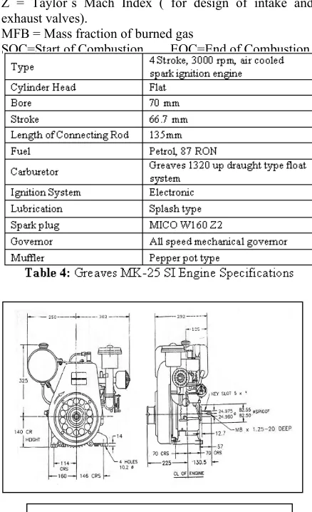
A fully computerized, variable compression
ratio, 4-Stroke, 256cc, 3000rpm, SI-Engine with electronic ignition control and a governor for speed control has been used for conduction of experiments pertaining to the above research. The compression ratio can be set to any value (even fractional values) with precision, as the test rig has a movable head under electronic motor control using a stepper motor and a precision manufactured Power Screw. In the present research, the compression ratio was varied as under, 4.63, 5.10, 6.0, 6.88, 7.40, 8.28, and 9.16. The experiments
New Empirical Correlations for Simulating the Influence
of Compression Ratio on Ignition Delay and Overall
Combustion Duration in SI Engines
have been conducted at Wide-Open-Throttle (WOT) conditions, and near stochiometric F/A ratios, unless otherwise mentioned. The rig also has a highly sensitive, water-cooled piezoelectric pressure sensor for accurate in cylinder pressure trace and temperature sensors for measuring temperature at strategic points in the operating cycle. The electronic ignition control system permits the ignition advance to be set for any operating conditions of the engine for maximum brake torque (MBT) conditions. Minor adjustments in the governor sleeve displacement and carburetor float level can be made for getting different fuel mixture strengths (or fuel equivalence ratios). A standard 16-bit data acquisition card connected to the personal computer handles all experimental data acquisition. The mass flow rate of air into the intake manifold is measured using an orifice provided on the intake plenum with a sensor fitted to it. The sensor sends the signal to data acquisition card which in turn is connected to the micro computer, for calculation of mass flow rate of air. The fuel flow rate is measured with the help of a sensor fitted to, the bottom of the fuel tank which senses the weight of the tank and calibrates it to give the fuel flow rate.
III AIR-FUEL (A/F) RATIO MEASUREMENT
The test rig has a sophisticated flow sensor mounted at the outlet of the fuel tank at its base, opening into a pipe that has a burette by its side provided with inlet and outlet taps near its bottom. The flow sensor provides an analog signal that is converted into a digital signal by the 1 bit A/D converter connected to the standalone 16 bit data acquisition card which communicates to the micro computer through the RS232 serial communication port.
The fuel flow rate could also be measured by the conventional method of letting the fuel from the fuel tank to fill up the burette by opening its inlet tap and closing it later while simultaneously noting down the volume of fuel consumed in certain period of time and determining the fuel flow rate.
The engine is equipped with an updraught type carburetor and the fuel equivalence ratios have been varied between 0.8 to 1.2 (approximately) by raising or lowering the carburetor float assembly with respect to the fuel nozzle.
Development of the Mathematical Model (experimental procedure) :
Despite the several limitations of the
Rassweiler and Withrow model for computing the MFB, which includes among others, its inability to account for crevice volumes, its sensitivity to selection of appropriate polytropic index during compression & combustion process, its inability to predict accurately the end of combustion (EOC), and its poor accountability of heat transfer effects, studies by researchers clearly points to the fact that it is still a preferred model for its simplicity and for its computationally undemanding requirements, while being almost as accurate as more complex models. In the present work therefore, this equation has been used for estimation of mass fraction burnt during combustion.
MFB =
∑
i0Pi
/∑
0n1Pi
= [(V*P 1/n1 – Vs*Ps1/n1) /
(Vf*Pf1/n1 – Vs*Ps1/n1)]
----1
The governor sleeve displacement and the carburetor float level were set to give near stochiometric F/A ratios when operating at WOT conditions. Log(P) vs.
Log(V) plots of the experimental P-θ trace were
obtained for different compression ratios keeping engine operating speed, constant.
The compression and expansion processes on
such a log-log diagram are nearly straight lines. The point where the above graph deviates sharply from the straight line representing the compression process was considered as start of combustion (SOC). Similarly, the point where the above log-log graph approaches sharply the straight line representing the expansion process was identified as the end of combustion (EOC). To improve the accuracy of determination of overall combustion duration using this conventional approach, the authors have replotted the graphs to several times
their normal size. The ‘scaled up’ graphs have been
graphically analyzed point by point (to an accuracy of ± 0.5º crank angle) and the slope at each of these points have been measured. The section of the graph where there is sharp difference in the slope between adjacent points
has been identified as ‘SOC’. ‘EOC’ has been
determined in a similar fashion. This approach provides not only a simple but an effective and accurate method to determine the overall combustion duration in the opinion
of the authors. The “Overall Combustion Duration”,
(crank angle between SOC and EOC), could therefore be
measured very accurately from the experimental P-θtrace
and the same is given in the form of table.
Table 1: Experimental values of overall combustion duration for varying compression ratio
Taylor’s equation which is very widely used
for determining the overall combustion duration in its original form is given as
∆θc =40+5*((n/600)-1)+(166* (((12.5/Y)-1.1)2))
Evidently this equation considers only the engine speed and equivalence ratio to determine the overall combustion duration expressed in terms of degrees of crank rotation. However from the graphs of figures (1 to 8), there is enough experimental evidence to suggest that the overall combustion duration indeed depends upon the compression ratio of the engine, as much as the other two factors. Taylor’s equation obviously predicts the same value for all the compression ratios (66deg). The error between the original equation and the experimental values as given in the above table are tabulated below.
r 4.63 5.10 6.0 6.88 7.40 8.28 9.16
Error 02 06 16 20 30 34 36
Table 2 : Error between the experimental values of overall combustion duration and that based on original Taylor’s equation
r 4.63 5.10 6.0 6.88 7.40 8.28 9.16
From the above table an error curve was fitted in the form of a logistic equation and the error in the original Taylor’s equation was minimized by incorporating this equation into it, thereby giving the modified Taylor’s equation.
∆θc=(40+(5*((n/600)-1))+166* (((12.5/Y)-1.1)2)-
(37.71/(1+(2411*exp(-1.2*r))))) ---2
Empirical flame combustion models have difficulty to appropriately describe the 3 phases of combustion, viz., the flame development phase, the rapid burn phase, the flame termination phase, with sufficient generality to be widely useful. Usage of 2-Zone model (burnt & unburnt regions being separated by a thin reaction flame sheet) together with coupled analysis of flame front location and cylinder pressure data, gives the following burning law which is used as a first step towards the model building. d/dt(mb)=ρu*Af*Sl + μ/τ ---3
Eqn-3, above when effectively integrated over the relevant portion of the total combustion process, assuming the turbulent characteristic velocity as proportional to mean piston speed, an equation for the flame development angle could be obtained as ∆θd = C*(Vp*γ)1/3*(h/S l)2/3 (C has to be evaluated)--4
The above equation as proposed by Keck et al., is applicable to SI engines in general but does not take into account the parameters related to engine geometry especially the location of the spark plug, swirl generation during intake process and the effect of compression ratio etc. In the present paper, the influence of the above parameters have been indirectly taken into account by fitting it with a “Polynomial Equation of the 3rd order”, by minimization of error using non-linear regression analysis. The evaluation of the constant “C”, in equation(4), has been done using this model and therefore, the authors believe, it must yield a more accurate prediction of the flame development phase in SI engine combustion. Slo = 0.263 + [ - 0.847*(Ф – 1.13)2]---5
α = 2.18 – [0.8*( Ф – 1 )]---6
β = -0.16 + [0.22*( Ф – 1)]---7
Sl = Slo*(Ti/298) α * (p /1030000) β---8
Equations 5,6,7,8 are used to evaluate the laminar flame speed (Sl), which upon substitution in equation (2), enables C to be evaluated if experimental values of ∆θd are available. The experimental values of ∆θd was found from the point of ignition to the point where an appreciable rise in cylinder pressure was noticeable, from the motored P-θ curve superimposed on the engine firing P-θ diagram ∆T = hfg / [(A/F)*Cpa + Cpf] ---9
∆P= -pi*k*∆V/V+(p3-p2)*(Vtdc/Vi)* [(d/dt)MFB]--10
MFB= 1 – exp(-a*((θ – θi)/∆θc)m+1) --- --11
hcW = 3.26*B - 0.2 *∆P 0.8 * T - 0.55* Vg 0.8 ---12
k = kr + ( kp + kr)* [(d/dt)MFB]--- --13
Equation (9) is used to calculate the drop in temp at Intake manifold due to fuel vaporization. Equation (10) is used to calculate the rise in cylinder pressure if mass fraction burnt (MFB) is known or conversely to evaluate
(MFB) from experimental P-θ diagram. Equation (11) is
the Weibe model. Equation (12) is the Woshni`s relation to evaluate the instantaneous heat transfer during combustion. Equation (13) gives variability in the polytropic index during combustion & expansion.
The motored P-θ trace was obtained for these
settings. Spark advance was adjusted to MBT
(corresponding to lowest SFC) and the corresponding P-θ
trace was obtained, under WOT firing conditions. The flame development angle was established by super
imposing the motored P-θ diagram over the
corresponding P-θ diagram obtained under firing
conditions for MBT setting of the spark advance for the given compression ratio. The above value of flame development angle was used as a basis for calculating the tentative value of the constant “C”, in equation(4). This equation is the revised equation which still does not account for either the compression ratio or the F/A equivalence ratio
The compression ratio was varied and for
each compression ratio setting, the spark advance was set for MBT and the flame advance angle were determined as explained in the previous step and the results obtained were tabulated.
With the revised version of equation (4), simulation was carried out by incorporating the same and running the program. The values predicted by the C-program with the revised equation(4) and the experimentally obtained values of the flame development angle (MBT setting), are tabulated below.
Table3: Experimental and Simulated values of flame development angle (FDA) and error
The error between the experimental &
simulated values of the flame development angle were
minimized and a polynomial equation of 3rd order was
fit into the revised equation(4).
The governor setup was detached from the
∆θd = C*(Vp*γ)1/3*(h/S
l)2/3 – (( -3.129*r) + (0.9894*r2) - (0.06508*r3))---14
IV RESULTS AND DISCUSSION:
The graphs of Figures 1 – 8, show the plot of
Log(P) vs. Log(V), from the experimental P-θ trace
depicting the start of combustion (SOC) and end of combustion (EOC), for various compression ratios and for conditions where intake generated swirl in the intake manifold is present or not present. From a perusal of the graphs, it is clear that both compression ratio and intake generated swirl have a considerable influence on the overall burn duration during the combustion process, with the influence of compression ratio being more predominant.
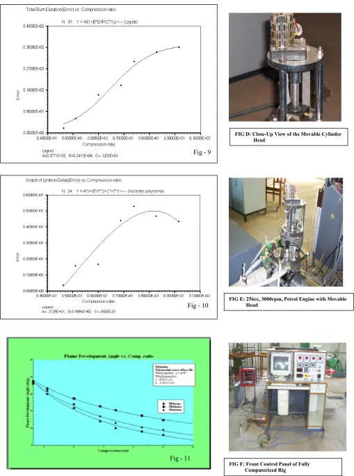
The graphs of Figure 9 and 10 show the plot of
error vs. compression ratio for overall combustion duration and ignition delay respectively, based on the actual experimental values and that obtained under simulation using the premodified Taylor’s equation for combustion duration and Keck’s equation for ignition delay. This error has been minimized by incorporating them in these equations thereby leading to their respective modified forms which have been discussed in the previous topic.
The graphs of Fig-11 show the improvement in
the prediction of the ignition delay as the original Keck’s equation is modified in two stages, by taking the influence of the compression ratio of the engine and later the fuel mixture strengths (or equivalence ratio) into account. This equation is also used to optimize the performance of the SI engine as it gives a measure of the optimum spark advance needed by simulating for MBT conditions of operation. The authors believe this to be true since the modified equation for the flame development angle is based on MBT setting of the engine when operating at various compression ratios.
V CONCLUSIONS:
1. The authors in this paper have made an attempt to improve the combustion simulation models particularly the empirical equations that are used to predict the Overall Combustion Duration and Ignition Delay for a more realistic simulation.
2. The equation proposed by Taylor to predict the overall combustion duration has been improved by including the influence of compression ratio, and the modified equation is
∆θc=(40+(5*((n/600)-1))+166*pow(((12.5/Y)- 1.1) 2)- (37.71/(1+(2411*exp(-1.2*r)))))
3. The equation propounded by Keck and coworkers to predict the flame development angle in SI engines has been improved by including the influence of compression ratio as ∆θd = C*(Vp*γ)1/3*(h/S
l)2/3 – (( -3.129*r) + (0.9894*r2) - (0.06508*r3)))
4. From purely theoretical considerations, the performance of SI engines could be optimized by appropriately computing the ignition delay and setting the spark advance angle to correspond approximately to this value, under WOT operating conditions. This effectively ensures that peak cylinder pressures occur just after TDC thereby optimizing the work output of SI engines as it reduces the compression work and enhances the work done during the combustion.
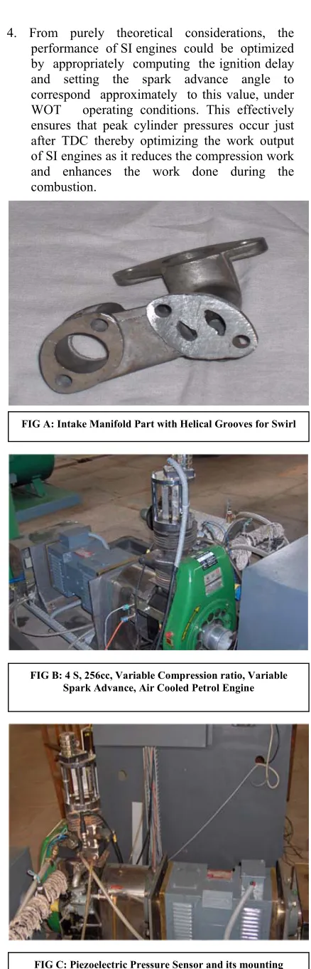
[image:4.612.335.554.30.711.2]FIG A: Intake Manifold Part with Helical Grooves for Swirl
FIG B: 4 S, 256cc, Variable Compression ratio, Variable Spark Advance, Air Cooled Petrol Engine
[image:4.612.340.554.356.705.2]Fig -0 0.2 0.4 0.6 0.8 1 1.2 1.4 1.6
1.75 1.85 1.95 2.05 2.15 2.25 2.35
Log10(V)
Log1
0(
P
)
Comp. Ratio = 4.63, Comb. Duration = 64deg.
SOC EOC Fig - 0 0.2 0.4 0.6 0.8 1 1.2 1.4 1.6
1.75 1.85 1.95 2.05 2.15 2.25
Log10(V)
Log10
(P)
Comp. Ratio = 5.1, Comb. Duration = 60deg
SOC EOC Fig -0 0.2 0.4 0.6 0.8 1 1.2 1.4 1.6
1.75 1.85 1.95 2.05 2.15 2.25
Log10(V)
Lo
g10(
P
)
Comp. Ratio = 6.0, Comb. Duration = 50deg.
SOC EOC Fig -0 0.2 0.4 0.6 0.8 1 1.2 1.4 1.6
1.5 1.6 1.7 1.8 1.9 2 2.1 2.2
Log10(V) Log 1 0 (P )
Comp. Ratio = 6.88, Comb. Duration = 46deg.
SOC EOC Fig - 0 0.2 0.4 0.6 0.8 1 1.2 1.4 1.6
1.8 1.9 2 2.1 2.2 2.3
Log10(V)
Log1
0
(P)
Comp Ratio = 4.63, Comb. Duration = 54deg
EOC SOC With Swirl Fig - 0 0.2 0.4 0.6 0.8 1 1.2 1.4
1.75 1.85 1.95 2.05 2.15 2.25
Log10(V)
Log1
0(
P)
Comp. Ratio = 5.1, Comb. Duration=52deg.
With Swirl SOC EOC Fig - 0 0.2 0.4 0.6 0.8 1 1.2 1.4 1.6
1.65 1.75 1.85 1.95 2.05 2.15 2.25
Log10(V)
Log1
0
(P
)
Comp. Ratio = 6.0, Comb. Duration = 46deg
With Swirl SOC EOC Fig -0 0.2 0.4 0.6 0.8 1 1.2 1.4 1.6
1.6 1.7 1.8 1.9 2 2.1 2.2 2.3 2.4
Log10(V)
Lo
g1
0(
P)
Comp. Ratio = 6.88, Comb. Duration = 36deg.
With Swirl
SOC EOC
Fig - 1 Fig - 2
Fig - 3 Fig - 4
Fig - 5 Fig - 6
Fig - 9
Fig - 10 FIG E: 256cc, 3000rpm, Petrol Engine with Movable Head
[image:6.612.61.570.67.751.2]FIG F: Front Control Panel of Fully
FIG D: Close-Up View of the Movable Cylinder Head
VI REFERENCES:
[1] Annand W.J.D. “A new computation model for combustion in SI-Engine”, Proc., I.Mech.E., Vol 185, Nov 1971. [2] Blizard N.C. and Keck J.C., “Experimental & Theoretical
Investigation of Turbulent Burning Model for IC-Engines”, SAE Paper 740191, SAE Automotive Engineering Congress, Detroit, Feb 1974.
[3] Ball J.K. et al. “Combustion analysis and cycle by cycle variation in SI-Engine combustion”, “Part1-An evaluation of combustion analysis routines by reference to model data”, Proc., I.Mech.E., Vol212..
[4] Pischinger S. and Heywood J.B., “A model for Flame kernel development in an SI- Engine”, 23rd International
Symposium on Combustion, 1990.
[5] Hinze P.C. and Heywood J.B., “A model for flame initiation and early development in SI-Engines & its application to cycle to cycle variations”, paper 942049, SAE, pp1808-1815, 1992.
[6] Hinze P.C. and Heywood J.B., “A study of cycle to cycle variation in SI-Engines using a modified quasi dimensional model”, SAE paper 961187, 1996.
[7] Jensen J.K. and Schramm J., “ A Three Zone Heat release Model for combustion analysis in a natural gas SI-Engine— Effects of Crevices and cyclic variations on UHC emissions”, Paper 200-01-2802, SAE, 2000.
[8] Heywood J.B., Higgins J.M., Watts P.A., Tabaczynski R.J., “Development & use of cycle simulation to predict SI-Engine Efficiency & Nox emissions”, SAE paper, 79021, 1979.
[9] Gautam K. Kalghatgi, “Spark Ignition, Early Flame development & cyclic variation in IC-Engines”, SAE Technical Paper Series, 870163,International Congress & Exposition, Detroit, Michigan, Feb 23-27, 1987.
[10] Kyuy Hwan Lee and David E.F., “Cycle by cycle variation in combustion and mixture concentration in the vicinity of the spark plug”, SAE paper 950814.
[11] Harish Kumar R. and Antony A.J., “A Simple Approach to Predict Ignition Delay for Optimising SI-Engine Performance”, paper no. IN_13, “3rd BSME-ASME
International Conference on thermal Engineering”, 20th
to 22nd December 2006, Dhaka, Bangladesh.
VI SYMBOLS (SI UNITS) & ABBREVIATIONS
∆P = Instantaneous cylinder pressure change during
combustion.
∆T = Intake manifold temperature.
∆θc = Total combustion duration specified in terms of
crank angle.
θ = Instantaneous Crank angle
∆θd = flame development angle/ignition delay
θi = Crank angle at the point of ignition
Ф = Fuel equivalence ratio (EQR)
ρu , ρb = density of unburnt and burned gas respectively.
Β = Cylinder Bore Cpa = Specific heat of air.
hcW = Instantaneous heat transfer coefficient), based on Woschni`s equation.
n = engine speed, rpm.
hfg = Heat of vaporization of the fuel.
Vd = displacement volume of the cylinder h=clearance height at the point of ignition
k=Effective polytropic index of compression/expansion during progressive combustion.
kp = polytropic index of expansion for product gases. kr = polytropic index of compression/expansion for reactant mixture
m = Mass of charge with suffixes u & b denoting unburnt and burnt fractions.
MFB= Mass fraction of burnt gases during progressive combustion.
l t = Characteristic length(equal to bore)
V, P = Instantaneous cylinder volume and pressure during combustion with suffix i denoting instantaneous values. p2 , p3 = Theoretical cylinder pressure at end of compression and combustion respectively.
Sl = Laminar flame speed. Slo, α, β, = Parameters
used in equation 8, to find laminar flame speed. T = Temperature (in deg K) with suffixes.
Vtdc, = Cylinder volume at TDC. Vg = Gas velocity during combustion
Vs , Ps ,Vf , Pf = cylinder volume and cylinder pressure at the start of combustion and end of combustion respectively. ls=stroke length
Vi = Instantaneous cylinder volume at any crank angle. n1 = total crank angle intervals for complete combustion. Y = Number of moles of actual oxygen supplied to the engine. lc=Length of connecting rod Ycc = Number of moles of chemically correct oxygen requirement during combustion.
r = Compression ratio. rc = crank radius
γ = Kinematic viscosity
i = suffix to designate instantaneous value or the start of ignition.
ξ = Characteristic burning time (l t / Sl )
μ = Parametric mass entrained within the flame region
that has yet to burn.
Z = Taylor`s Mach Index ( for design of intake and exhaust valves).
MFB = Mass fraction of burned gas
[image:7.612.322.541.367.726.2]SOC=Start of Combustion. EOC=End of Combustion