Abstract— Modern marine vessels perform a wide spectrum of various tasks, including the most difficult research efforts and rescue expeditions. So, the problem of construction of automatic motion control systems for them has received considerable attention in various scientific publications. One of the most important requirements to any control system is the availability of the property of astaticism on regulated coordinates, i.e. the systems’ ability to provide zero static error when exposed to the constant external disturbances. At that the astaticism property should be performed not only in the stabilization mode of the motion of an object, but also in the functioning of the object in the other modes of motion. Significant attention in this paper is paid to the motion control laws in a predetermined path with the multipurpose structure, providing astaticism of the closed-loop system. In the paper the method to provide the astaticism in tracking control system is proposed, described in details and examined on the example.
Index Terms— control law, observer, stability, tracking control, astaticism
I. INTRODUCTION
URRENTLY, the problem of construction of automatic motion control systems for moving objects, particularly for marine vessels, performing a wide spectrum of various tasks, has received considerable attention in various scientific publications. This is due to the continuous expansion of the range of requirements to such systems, and the growing capabilities of the devices that implement the control laws.
In this regard, there is a need to use multipurpose control laws, allowing taking into account the complex of conditions, requirements and restrictions that must definitely be performed in all modes of operation of the rolling object. Such onboard systems give a great number of advantages that are not possible in manual control mode. These benefits include speed of processing data, the completeness of the considered factors, the accuracy of testing a given trajectory, the selection of the optimal settings, etc.
In connection with this circumstance, to ensure all required dynamic properties of any moving object there must be some compromise on quality control processes in
Manuscript received December 6, 2015; revised January 3, 2016. M. A. Smirnova is with the Faculty of Applied Mathematics and Control Processes, Saint-Petersburg State University, 7/9 Universitetskaya nab., St. Petersburg, 199034, Russia (e-mail: [email protected]).
M. N. Smirnov is with Faculty of Applied Mathematics and Control Processes, Saint-Petersburg State University, 7/9 Universitetskaya nab., St. Petersburg, 199034, Russia (e-mail: [email protected]).
T. E. Smirnova is with the Faculty of Applied Mathematics and Control Processes, Saint-Petersburg State University, 7/9 Universitetskaya nab., St. Petersburg, 199034, Russia (e-mail: [email protected]).
N. V. Smirnov is with the Faculty of Applied Mathematics and Control Processes, Saint-Petersburg State University, 7/9 Universitetskaya nab., St.
different modes. Obviously, the simplest way is to build a single control law, which will provide admissible quality of motion in any mode, but for each of them separately specified control law will be far from the optimal one.
Note that for most individual modes of motion numerous methods for the synthesis of control laws [1-5], effective for specific situations, are developed. The multipurpose control laws that are focused on a set of modes are studied much less. These circumstances may create additional difficulties in the design of automatic control systems of moving objects.
One of the most important requirements to any control system is the availability of the property of astaticism on regulated coordinates, i.e. the systems’ ability to provide zero static error when exposed to the constant external disturbances. At that the astaticism property should be performed not only in the stabilization mode of the motion of an object, but also in the functioning of the object in the other modes of motion.
In particular, significant attention in this paper is paid to the motion control laws in a predetermined path with the multipurpose structure, providing astaticism of the closed-loop system. Some methods to provide the astaticism are described in [6-10].
Works [11-20] present the theory of multipurpose synthesis of motion control systems, taking into account the complex set of conditions, requirements and restrictions which certainly should be performed in all operation modes of the vessel.
II. TRACKING CONTROL PROBLEM
An easy way to comply with the conference paper formatting In many practically important situations (obstacle avoidance, motion in narrow corridors, performing various maneuvers and group movement, and so on), the control system implements automatic maneuvering by practicing the given command signal yd(t), i.e., by ensuring the closeness of the values of real output y(t) of the closed-loop system to the desired value yd(t) of output at each moment
] , 0 [ T
t of the maneuvering process.
Note that identical coincidence of these functions is almost impossible due to the inertia of the object, limited control resources, errors in measurements and etc. However, we assume that a given motion is realizable in the sense that here exists a feedback control law, which will provide in a closed-loop system the condition
) ( ) (t yd t
y , t. (1)
Let consider some implementation issues of tracking control with the multipurpose structure using a linear stationary object with a mathematical model
Astaticism in Tracking Control Systems
Maria A. Smirnova, Mikhail N. Smirnov, Tatyana E. Smirnova, Nikolay V. Smirnov
,
, (0)
, 0
Du Cξ y
ξ ξ Bu Aξ ξ
(2) where ξEν is a state vector, uE is a control vector,
k
E
y is a vector of regulated coordinates, A, B, C, В are constant matrices with corresponding dimensions.
Equations (2) are determine the linear stationary operator
Y U
p
: , ypu, (3) that at given initial conditions on the state vector establishes a one-to-one correspondence between each control u from the set U and each output y from the set Y. Further, we will assume that the corresponding inverse operator p1 is defined.
Let the stabilizing feedback with LTI (Linear Time Invariant) mathematical model is given
, , y D ζ C u
y B ζ A ζ
c c
c c
(4) where ζEν1 is a state vector of controller, A
c, Bc, Cc, Dc
are constant matrices with corresponding dimensions. Note that the initial conditions for vector ζ are always assumed to be zero.
As for the controlled object, the linear stationary feedback operator corresponds to the model (4)
U Y
c
: , ucy. (5) Operator (5) establishes a one-to-one correspondence between each output y from the set Y and each control u from the set U.
Let consider the closed-loop system (2), (4). In accordance with the relations (3) and (5) we have
y
ypc (6)
i.e. the equation, which solution leads to a linear stationary operator 3 of the closed-loop homogeneous system, is
0 3
y . (7)
Since the feedback is stabilizing, zero equilibrium position of system (7) is asymptotically stable by Lyapunov, i.e. the condition (8) is fulfilled
0
y(t) at t for any ξ0Eν. (8) Now, instead of feedback (5) we form the control action as the following sum
d
c d
py y y
u1 (9)
where the first term can be interpreted as command signal )
( )
(t p1yd t
u , fed to the closed-loop system, and the second term u~c
yyd
represents the feedback with the tracking error e(t)y(t)yd(t).Subject to the linearity of the operator p, the closed-loop system (3), (9) is
) ( )
( d d p c d
c p
d y y y y y y
y
y
or epce. According to (6) and (7) we have the closed-loop homogeneous system
0 3
e (10)
It is easy to see that if the initial conditions ξ
0 ξ0 on the state vector of the object are non-zero, the left side of (10) will have an additional term e0(ξ0), which tends exponentially to zero with unlimited growth of time. Then, due to asymptotic stability, we have0
e(t) at t for any ξ0Eν. (11) which implies the condition
) ( ) (t yd t
y at t.
Let concretize this scheme to implement the desired motion in a given direction using a stabilizing control according to the state of the object.
Consider the linear mathematical model of the moving object with linear actuator:
. ,
,
Cx y
u δ
Bδ Ax x
(12)
Here xEn is a state vector, δEm is a vector of control actions, uEm is a vector of control signals (controls), yEk, kn is an output of the system.
Let consider the situation when C
0 C2
, where C2 is non-singular square nn matrix, i.e. the following equality is valid:
2 22 1
2 C x
x x C 0 Cx
y
,
k E
2
x , detC20.
(13)
Let also consider the equation of stabilizing state control δ
K x K
u x , (14)
that due to the notation Kx
Kx1 Kx2
can be written asδ K x K x K
u x1 1 x2 2 . With subject to (13), let denote
y K y C K x K
v 1
1 2 2 2
2
x
x ,
1 2 2 1
K C
K x . (15)
Then we can write the auxiliary LTI system with the input v and the output y
.
, ,
1 1
Cx y
δ K v x K δ
Bδ Ax x
x
(16)
In block representation these equations will take the form
, ,
ξ C y
v B ξ A ξ
p p p
(17) where
m n
E
δ x
ξ ,
K 0 K
B A
A
1 x
p ,
m p
E 0
B , Cp
C 0
. After recording (17) in tf – form we obtain, ) ( v H
y s (18)
where transfer matrix H is
) ( ) ( )
(s Ba s Aa s
H , (19)
p
a s s
A( )detE A ,
p
pp a
a s A sC Es A B
B ( ) ( ) 1 , (20)
with the identity (nm)-matrix E.
With account to (18) and (15) the equations of the closed-loop system (12), (14) can be written in operator form
, , , ) ( ) (
1 p d dt
p p
Aa a
y K v v B y (21) which determine respectively the operators p and c specified higher. Note that for the first one there exist the inverse operator p1, that is uniquely determined by inverse transfer matrix H1(s)Aa(s)Ba1(s) of the auxiliary system.
It is easy to see that equations (21) are reduced to a homogeneous system of differential equations relatively to the stable output
Aa(p)EkBa(p)K1
y0, (22) with hurwitzian characteristic polynomial (s). It is important to note that equation (22) specifies a uniform stationary operator 3 entered in the general case by (10).Now let's use the auxiliary stabilizing controller (15) to implement the desired motion yd(t) of the output. To this
end, in accordance with the formula (9) we generate the control signal in the following form
). ( ) ( 1 1 1 d d d c d ppy K y y
H v y y y v (23) Then the equations of the closed-loop system are
). ( ) ( , ) ( ) ( 1 1 d d a a p p p A y y K y H v v B y
(24)
Equations (24) can be easily reduced to one uniform equation
Aa(p)EkBa(p)K1
e0 (25) with respect to the tracking error e. Due to the characteristic polynomial of the system (22) is Hurwitz polynomial, the polynomial of the system (25) will also be Hurwitz polynomial. Thus, for any initial conditions ξ(0)ξ0 on the state vector of the object (12) with actuator, on the basis of (25) have
y y
0et t d t , t.
So we can formulate the transformation rule of the given stabilizing control to realize the desired motion of the controlled object:
()
.) ( )
( 1 1 2 21
1 2 2 1 1 δ K y y C K x K y H u δ K x K x K δ K x K u t t
p d x x d
x x x
(26)
Here the first term u*(t)H1(p)yd(t) can be interpreted as command signal, fed to the closed-loop system, and the second term
y y
K δC K x K
u~(t) x1 1 x2 21 d(t)
represents the feedback with the tracking error )
( ) ( )
(t yt yd t
e .
Let consider the system with constant external disturbance
t1 0 d d
. , , Cx y u δ Dd Bδ Ax x t (27)Assume, that we have the basic control law δ
K Kx
u 0 . On its basis let construct the control law in
the form
y z μ
u , (28)
where z is the estimation of the state vector, obtained using the asymptotic observer
y Cz
GBδ Az
z . (29)
In static equilibrium position the equalities
0 , 0 ,
0
δ z
x are fulfilled. Thus, we have
, 0 , 0 y Bδ Ax
and, consequently, y0. So the structure of the control law (28) provides the astaticism of the closed-loop system.
Let transform the controller (28) to realize the desired motion yd
t . The controller (28) can be represented in theform , y δ K x K z K
u z x (30)
where KzμAμGC, KμB, ΚxμGC.
Then the closed-loop system (27), (29), (30) can be written as
. , , Cz y G Bδ Az z x C K δ K z K δ Dd Bδ Ax x x z t (31)Let denote the state vector of the system (31) as
nm x,δ,z ,dimξ 2
ξ .
The condition of astaticism on ith controllable coordinate for the system (31) can be represented in the following form
0 0, id
H (32)
where
s i
d
H is a transfer function of the system (31) from the disturbance d
t to ith controllable coordinate.
si
d H
is determined by formula
det ,, 1 1 2 1 GC A E B 0 K K E 0 0 B D H H 0 0 H d d d s s s s s s z i m n i i (33)
where
s is a characteristic polynomial of the system (27), (28).Thus, the problem of providing astaticism of the closed-loop system on the controlled coordinates is reduced to the choice of the matrices μ,ν in regulator (28), to satisfy the conditions (32).
Similarly we can formulate the transformation rule of the given stabilizing astatic control (28) to realize the desired motion of the controlled object:
.1
d d
py z y y
H
III. SYNTHESIS OF THE CONTROLLER
Let consider the system of automatic tracking control with respect to the requirement of astaticism.
Consider the mathematical model of marine vessel:
. δ
, ω
); ( δ ω β ω
); ( δ β β ω β β
2 2 2 2 1
1 1 0 1 2 1 1
u
t M b a a
t F b a a a
(35)
Here is the angular velocity relative to the vertical axis,
is a yaw, is the deviation angle of vertical rudders, is the drift angle, u is a control, Fh1f(t) is a side force,
) (
2f t
h
[image:4.595.46.286.257.394.2]M is a moment, f(t) is an external stepwise disturbance, determined by wind and waves. The marine vessel used for modelling is shown in Fig.1.
Fig. 1 Marine vessel
Let’s take harmonic oscillation d(t)Adsindt with
the given amplitude and frequency as program motion. Then, according to (34), the transformation rule for the given stabilizing control
1 2 3 u
is as follows
μ μ μ
,, ) ( ν )
( ) (
), ( δ
3 2 1
1
μ
z μ
cz g b Az z
t t
p H
u d d
where coefficients are
. 4062 . 0 ν , 2482 . 4 μ , 9414 . 6 μ , 7068 . 1
μ1 2 3
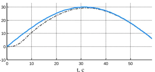
The corresponding dynamic process for specified program motion d is presented in Fig. 2. The graphs show that when using speed controller the vessel reach the desired trajectory.
0 10 20 30 40 50 60
-10 0 10 20 30
t, c и
d, град
Fig. 2. Adjustment of the program motion. Desired trajectory (dashed line)
In Fig. 2 solid line represents the desired trajectory and dashed line – current position of the marine vessel. As shown in the Fig. 2, the vessel needs only 30 seconds to reach the given trajectory d. As follows from the example the control law (34) provides zero tracking error, i.e. the system with controller (34) is astatic on yaw.
Represented algorithm is implemented in the environment MATLAB with the subsystem Simulink. MATLAB is one of the most effective tools to form and use in the researches computer models of dynamic systems. So the realization of this algorithm can be easily used for any controlled object.
IV. CONCLUSIONS
Following the given trajectory is related to the necessity to avoid obstacles, vessels’ movement in narrow waters, performing the maneuvers of divergence and group motion of marine vessels and etc. In these situations the program of yaw motion d(t) is specified, and the control problem is to
provide the proximity of current yaw values (t) and desired yaw d(t) at every time moment t0. At the same
time the property of astaticism is very important to provide zero stabilization error in the process of any complicated motion.
In the paper the method to provide the astaticism in tracking control system is proposed, described in details and examined on the example.
REFERENCES
[1] Fossen T. I. Guidance and Control of Ocean Vehicles. John Wiley & Sons. New York, 1994.
[2] Fossen T. I. Handbook of Marine Craft Hydrodynamics and Motion Control. John Wiley & Sons, Ltd., 2011.
[3] Smirnov N.V., Smirnova M.A., Smirnova T.E., Smirnov M.N. Multiprogram digital control. Lecture Notes in Engineering and Computer Science. Vol. 1. pp. 268–271, 2014.
[4] Smirnov M.N., Smirnova M.A., Smirnov N.V. The method of accounting of bounded external disturbances for the synthesis of feedbacks with multi-purpose structure. Lecture Notes in Engineering and Computer Science. Vol. 1. pp. 301–304, 2014. [5] Smirnov M.N., Smirnova M.A. Dynamical Compensation of
Bounded External Impacts for Yaw Stabilisation System. The Proceedings XXIV International Conference on Information, Communication and Automation Technologies. pp. 1-3, 2013. [6] Smirnov M.N. Suppression of Bounded Exogenous Disturbances Act
on a Sea-going Ship. Proceedings of the 13th International Conference on Humans and Computers. pp. 114-116, 2010. [7] Smirnova M.A., Smirnov M.N., Smirnova T.E. Astaticism in the
motion control systems of marine vessels. Lecture Notes in Engineering and Computer Science. Vol. 1. pp. 258–261, 2014. [8] Smirnova M.A., Smirnov M.N. Synthesis of Astatic Control Laws of
Marine Vessel Motion. Proceedings of the 18th International Conference on Methods and Models in Automation and Robotics. pp. 678-681, 2013.
[9] Smirnova M.A., Smirnov M.N. Modal Synthesis of Astatic Controllers for Yaw Stabilization System. The Proceedings XXIV International Conference on Information, Communication and Automation Technologies. pp. 1-5, 2013.
[10] Fedorova M.A. Computer Modeling of the Astatic Stabilization System of Sea-going Ship Course. Proceedings of the 13th International Conference on Humans and Computers. pp. 117-120, 2010.
[image:4.595.50.297.635.750.2][12] Veremey E.I. Synthesis of multiobjective control laws for ship motion. Gyroscopy and Navigation, 1 (2), pp. 119 – 125, 2010. [13] N. V. Smirnov, T. E. Smirnova, “The stabilization of a family of
programmed motions of the bilinear non-stationary system,” Vestnik Sankt-Peterburgskogo Universiteta. Ser 1. Matematika Mekhanika Astronomiya, vol. 2, no. 8, pp. 70–75, Apr.1998 (in Russian). [14] N. Smirnov, “Multiprogram control for dynamic systems: a point of
view,” in Proceedings of the 2012 Joint International Conference on Human-Centered Computer Environments, HCCE'12, Aizu-Wakamatsu & Hamamatsu, Japan, Duesseldorf, Germany, March 8– 13, 2012. pp. 106–113.
[15] N. V. Smirnov, T. E. Smirnova, Ya. A. Shakhov, “Stabilization of a given set of equilibrium states of nonlinear systems,” Journal of Computer and Systems Sciences International, vol. 51, Iss. 2, pp. 169–175, Apr. 2012.
[16] N. V. Smirnov, “A complete-order hybrid identifier for multiprogrammed stabilization,” Automation and Remote Control, vol. 67, no. 7, pp. 1051–1061, Jul. 2006.
[17] Veremey E.I., Smirnova M.A., Smirnov M.N. Synthesis of Stabilizing Control Laws with Uncertain Disturbances for Marine Vessels. Proceedings of The 2015 International Conference "Stability and Control Processes" in Memory of V.I. Zubov (SCP), Russia, Saint-Petersburg, October 5 – 9, pp.1 – 3, 2015.
[18] Arzumanyan N. K., Smirnova M.A., Smirnov M.N. Synthesis and modeling of anti-lock braking system. Proceedings of The 2015 International Conference "Stability and Control Processes" in Memory of V.I. Zubov (SCP), Russia, Saint-Petersburg, October 5 – 9, pp.552 – 554, 2015.
[19] Smirnov N.V., Smirnova M.A., Smirnova T.E., Smirnov M.N. Modernization of the Approach for Bounded External Disturbances Compensation. Proceedings of The 2015 CACS International Automatic Control Conference, 2015.