Abstract— Sliding mode is an acknowledged nonlinear
robust control method which suffers from chattering phenomenon, the destructive high-frequency oscillations in internal states and control signal. One of the suggested routines to reduce chattering is to replace the discontinuity switching term, in standard method formulation, with a saturation function. Considering the fact that saturation function, with fixed-gradient, reduces the performance; we utilize an adaptive-gradient saturation function to overcome this limitation. Reinforcement learning algorithm is employed to find the instantaneous optimal value for the gradient of saturation function, with the ultimate goal of chattering reduction. The proposed intelligent sliding mode controller is applied to the tracking problem of chaotic Lorenz plant whereas the agent is rewarded (punished) for lower (higher) chattering. Simulation results are reported for standard and intelligent sliding mode controllers. The efficient control signal density as well as lower tracking error was attained after the agent learned the dynamics of the complex chaotic plant. Incorporating reinforcement learning into robust nonlinear control theory shows a promising route to achieve better performance.
Index Terms— Sliding mode control, Reinforcement
learning, Chattering reduction, Controlling chaos.
I. INTRODUCTION
liding-mode control is a subset of variable structure control methods due to uneven interactions in different regions of state space. Although this variability enhances robustness with respect to parameter uncertainties and un-modelled dynamics, it causes the undesirable chattering problem. Chattering is the high frequency oscillations, present in all system states, which causes low control accuracy, high wear of mechanical parts and heat loss in power electrical circuits. To overcome this detrimental phenomenon, a number of different techniques have been proposed during the last decades [1-3]. In these early works, authors replaced the discontinuous term by smooth functions, which reduced the chattering to the extent possible, however it resulted in poor error performance. The realization of chattering reduction and error convergence was addressed in a class of nonlinear systems using internal model principle [4]. The use of higher order sliding mode controller by replacing the higher derivatives of the control signal was proposed in [5]. Using auxiliary observer loop to A. B. F. is with the Bioengineering Program, College of Engineering, Northeastern University, Boston, MA 02115 USA (phone: 617-373-7733; e-mail: [email protected]).
M. J. Y. is with School of Electrical and Computer Engineering, University of Tehran, Tehran, Iran (e-mail: [email protected]).
B. S. is with the Department of Electrical and Computer Engineering, Northeastern University, Boston, MA 02115 USA (e-mail: [email protected]).
lock the chattering in the internal loop was also proposed to reduce the chattering [6]. However this method mainly suffers from complex usage of observers and differential inequalities. Accordingly reduced-order observer for chattering reduction was proposed in [7]. A more recent study showed the effectiveness of low-pass filtering on control signal which can reduce chattering even in noisy environment [8].
Reinforcement learning (RL) is a psychologically inspired machine learning method that is widely acknowledged in game theory, control theory and optimization problems. This method introduces a framework to address how an agent takes actions in an environment to maximize a particular reward function [9]. RL was identified computationally efficient in adaptive optimal control systems; that deals with finding the best solution to extremize a function of the controlled process [10]. In [11] authors derived optimal controllers based on different reinforcement learning methods for class of linear time-invariant deterministic systems. The proposed algorithms were not based on any knowledge of the system dynamics and it only required system output feedback to converge to optimal solution. Incorporating RL into hybrid control architecture for solving online optimal tracking problem was studied in a partially-known linear time varying process [12]. The control law was dynamically scheduled between stabilizing nonlinear controller, to ensure stability, and RL agent, to provide optimal long-term performance. Results showed the tracking performance of the hybrid controller was improved over that of fixed structure controller.
Sliding mode control has been effectively investigated in control problem of high-complexity nonlinear processes including chaotic structures [13-4]. While this was practiced especially as state stabilization and regulation, less attention was paid to the more complex tracking problems. The Lorenz system is a benchmark complex nonlinear equation that occasionally exhibits strange chaotic behavior [15]. This process was recruited in this study to validate the proposed controller.
The purpose of this contribution is to introduce an intelligent sliding mode controller by incorporating RL into the standard sliding mode control. Accordingly, the standard sliding mode control is overviewed and the integration of RL into this framework is explained. The discontinuous switching term in the standard sliding-mode formulation is replaced by an adaptive-gradient saturation function. The term adaptive refers to the fact of finding the best solution for the saturation function intelligently, so as to minimize the chattering amplitude. Using the exemplary chaotic Lorenz plant, the developed intelligent controller was
Application of Reinforcement Learning in
Sliding Mode Control for Chattering Reduction
Amir Bahador Farjadian, Mohammad Javad Yazdanpanah, and Bahram Shafai
examined in the tracking problem, while the control objectives were to track an exemplary sinusoidal trajectory and also reduce the chattering. Simulation results are provided to enable comparison between different control scenarios in terms of chattering amplitude and tracking error.
II. METHODS A. Sliding-Mode Control (SMC)
Sliding-mode control, considered as a robust nonlinear control design, has the ability to overcome uncertainties caused by different sources. This objective is achieved by introduction of sliding manifold, Eq. (3), and fluctuating around it. The solution is divided into two phases: a reaching phase and sliding phase. During the reaching phase, the trajectories in phase space are steered to reach the sliding manifold in a finite time and during the sliding phase they’re confined to this invariant set approaching the origin [16].
Without loss of generality we consider the following dynamical system: )] , ( )[ , ( ) , ( ) , ( ) , ( 2 1 u g f f a
(1)
where ηRp and ξRn-p and δ
i, i = 1, 2 represent uncertainty
terms. Here the control objective is to stabilize the origin (η, ξ) = (0, 0) while the case can be extended to regulation or tracking problem with particular transformations. The first step is to find a feedback law in order to stabilize η states. This task is done by smooth function φ(η) as to stabilize the origin of Eq. (2) asymptotically, subject to φ(0) = 0.
)) ( , ( )) ( , ( ) , ( ) , ( 1 ) ( 1 f f
(2)
and the following sliding manifold is constructed:
) (
z , (3) Now the control input is designed so as to reach in z, and stabilize the internal dynamics by means of ueq, Eq. (9), and
keep it on the surface thereafter by means of v, Eq. (8), during the sliding phase. The control input, u in (10), is explicitly calculated by using standard Lyapunov scheme.
2 z
V , (4)
) , ( ) ) , ( , , ( ) , ( ) , , ( 1 1 2
v g u g v
eq
(5)
0,1
, ( , ) 0 ; ) , ( ) , , ( k v kv (6)
b ( , ) ) , (
(7)
p i z
k
vi 1 sgn( i), 1
) , (
(8)
)] , ( ) , ( )[ , (
1
f f
g
ueq a
(9)
v g
u
u eq 1(,) (10)
The introduction of signum function in Eq. (8) injects high frequency switching term into the formulation. However the system hardware clocks cannot keep up with discontinuities in practice and results in chattering problem. This “zig-zag” curved phenomenon is the cause of several factors such as low control accuracy, heat loss and high wear in mechanical instruments as well as instability.
One of the suggested routines to reduce the chattering problem is to replace the discontinuity term with saturation function, Fig. 1.
elsewhere z sign z z f ; ) (
; (11)
-1
1
-1
1
Fig. 1. Saturation function to replace the switching term in standard sliding mode control formulation.
The proper selection of is a trade-off between control accuracy (N, N: large positive value) and chattering (0).
This fact supports the use of methods to approximate
adaptively and in response to the underlying system dynamics. Reinforcement learning algorithm is suggested to estimate the optimal value of in an interactive fashion. B. Intelligent Controller
Reinforcement learning (RL) is concerned with how an agent takes actions in order to maximize a reward function in an environment. In this framework, an agent learns to make optimal decisions based on the history of information, which was received by interaction with environment. A state signal that holds all relevant information to make the optimal decision is said to have Markov property. In this study, by using the properties of Markov decision process (MDP), we applied the Q-learning method to the optimal control problem of finding the slope for saturation function [17]. Q-learning is a fast adaptive subset of RL method [9].
RL algorithm is a way of mapping world states to actions, on purpose, so as to maximize the long term reward. This goal is achieved by means of learning through direct interaction with the world states. This method is described by a triple <s, a, r>, representing state, action and reward, in a finite state MDP. Through the learning period the agent makes decisions, takes actions and accordingly enters new states. Based on how optimal this new state is, with respect to the desired goal, the taken action would result in reward (or penalty). This reward signal provides a mean to train the agent throughout learning.
In the first step, finite number of possible actions will be defined to the agent. During learning period, the process of action-selection depends on agent learning policy. This policy can be more exploratory at early stage of learning by giving uniform chance of selection to all actions. At the end of learning period, this policy should be shifted toward more exploitation in order to make use of the acquired knowledge. In -greedy learning policy, the agent will choose between the best action, according to the past experience, or other actions. Accordingly while the probability of choosing the best action is 1-, the probability of choosing other possible actions will be .
Agent will be rewarded (or punished) by taking an action in a particular state, and entering to the new state. Consequently learning is done by weighting (or suppressing) actions at each state, as instructed by the reward signal. These action values will be written in Q-table and they will be updated as the agent visits different states, and takes different actions. Learning objective is to find a global policy π: SA to maximize the long term accumulated reward.
The rule of adaptation, for the contents of Q-table, is expressed as in Eqs. (12-13) below:
) , ( ) , (
max 1
1 a t t t
t Q s a Q s a
r
TD (12)
TD a
s Q a s
Q( t, t) ( t, t) (13) While t is a notation of time, Q(st, at) is the value of the
current action ‘at’ at the current state ‘st’. Temporal
difference error (TD-error), is proportional to the update value that must be reinforced to the current <state, action> value, i.e. it is mean of weighting the current action based on the prediction of the best action value in the next step. rt+1 is an immediate reward, corresponding to the taken
action, which is gained by entering to the new state st+1. is
learning rate, which determines to what degree the newly acquired value, for that specific cell in Q-table, should override the previous knowledge, 0<≤1. =0 does not let the agent learn, and =1 gives the highest importance to the most recent update. is a discounting factor to the future rewards, 0≤<1. Choosing =0 makes the agent opportunistic by only considering current reward and
=1leads to the long term high reward.
Thus, the algorithm for this method can be written as follows:
Initialize Q(s, a) arbitrarily
Initialize st
Repeat
Choose at from st using policy derived from Q(st,
at)
(e.g., -greedy)
Take action at, observe rt+1 and enter st+1
Update Q(st, at) according to 12, 13
st←st+1
Until st is terminal
III. APPLICATION
A. Chaotic Lorenz System
One of the most common chaotic models is the Lorenz system which is the Fourier expansion of the Navier-Stokes equations along two spatial directions. The fluid stream and resulting temperature differences are rephrased in terms of three-variable dynamic non-linear equations [15].
The chaotic Lorenz system was selected as a plant while for the sake of generality the unmatched disturbance was taken to be additive to the plant.
1 3 2 1 3
2 1 3 1 2
1 2
1 ( )
x y
d u bx x x x
x rx x x x
x x p x
(14)
where p, r and b are positive parameters representing Prandtl number, the Rayleigh number and a geometric factor (b = 8/3, p = 10, r= 28), d is selected as a white Gaussian matched disturbance, d(0,1).
The process output was taken as the first state while the desired trajectory was considered as follows:
) 2 sin( 1 . 0
2 t
yd (15) Both standard and intelligent sliding-mode controllers were applied to the chaotic plant. Equivalent chattering and tracking-error were quantified, as a control performance, and listed in Table I.
B. Standard SMC
Considering the following transformation the Lorenz system equations can be rewritten in regular form of Eq. (1) as:
) (
, 2 2 1
1
1 x z p x x
z (16)
) )
1 ( )
(( 1 2 1 3
3 p r p x p x x x
z
As demonstrated in Fig. 2 and Fig. 5(a), SMC could afford the control objectives in case of tracking error whereas the chattering problem still exists.
C. Intelligent SMC (ISMC)
In accordance with Q-learning notation, states were identified as a function of controller output, as defined in Eq. (10), and its derivatives, Eq. (17). Agent actions were defined as different values. The long term learning objective was chattering reduction. The agent was given a choice of actions [0:3], which would result in consequent reward or penalty.
u c u c u c
st (17) c′′, c′ and c were chosen with respect to their counterpart’s amplitude, output derivatives, so as to give those equal effects. According to Eq. (17), the lower states represent lower chattering and the upper states correspond to higher amount of the unwanted phenomenon. The number of states and actions were defined prior to each simulation, as reported in Table I, and they were partitioned equally.
990 992 994 996 998 1000
1.9 1.95 2 2.05 2.1
(a)
0 200 400 600 800 1000
0 0.05 0.1 0.15 0.2
(b)
[image:4.612.317.538.126.300.2]time(s)
Fig. 2. SMC performance, (a). Output, dotted line, and the desired trajectory, solid line, (b). Root mean squared of tracking-error.
With respect the definition of sates, the reward function was defined, as Eq. (18), so as to increase in the lower states, where the amplitude and frequency of the control input were less significant.
t t s
r 1 (18)
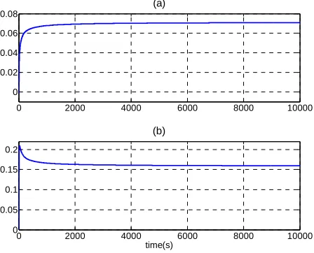
The agent average reward over the living period and root mean squared of Q-table variation, the TD-error, which is the learning index are illustrated in Fig. 4 as well. In this simulation, learning rate and discounting factor were chosen as =0.1 and =0.9999. Also In -greedy policy, was decreased monotonically toward the end of learning period, so that agent exploits the acquired knowledge the most at the end.
IV. RESULTS&CONCLUSION
Standard sliding mode control (SMC) and modified SMC (MSMC), which is formulated by fixed-gradient saturation function, were computationally simulated along with intelligent SMC. Outcomes were collected under equivalent
simulation parameters. The controllers were able to solve the tracking problem starting from random bounded initial conditions. The depicted long time running period was not necessary for the collected outcomes and it was selected to show the relative robustness and efficiency of the developed controller.
9990 9992 9994 9996 9998 10000
1.9 1.95 2 2.05 2.1
(a)
0 2000 4000 6000 8000 10000
0 0.05 0.1 0.15 0.2
(b)
[image:4.612.76.293.266.443.2]time(s)
Fig. 3. Intelligent SMC (agent 3) performance, (a). Output, dotted line, and the desired trajectory, solid line, (b). Root mean squared of tracking-error.
The problem was considered like the benchmark maze in reinforcement learning area where the agent was supposed to find a goal but in a dynamic environment. The RL agent performance is demonstrated in Figure 4. In this framework, the slope (in Eq. 11) of saturation function was estimated instantaneously by means of Q-learning algorithm. Fig. 4(a) demonstrates the total accumulated reward which follows an increasing trend up to almost fifth of the agent’s lifespan. The TD-error, in Eq. (12) and Fig. 4(b), is an indication of the reinforced signal to the agent. The asymptotic value of TD-error reflects the dynamic content of the chaotic plant that agent was unable to identify and cope with.
0 2000 4000 6000 8000 10000
0 0.02 0.04 0.06 0.08
(a)
0 2000 4000 6000 8000 10000
0 0.05 0.1 0.15 0.2
(b)
time(s)
Fig. 4. Agent 3 learning process, (a). Accumulated reward, (b). Root mean squared of TD-error.
[image:4.612.313.537.484.665.2]
02
) (
d
RMS (19)
Table I demonstrates the performance index of different controllers by integrating the RMS of tracking error (e) and the switching term (v), as in Eq. (8), which represents the chattering amplitude.
In development of the intelligent controller, variety of conditions were investigated based on the number of actions, states and the learning periods, as listed in Table I. Accordingly augmenting the Q-table dimension, which results in increased number of possible states and actions, improves the outcome performance but also exponentially increases the computational cost and convergence time.
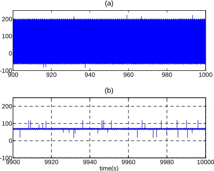
900 920 940 960 980 1000
-100 0 100 200
(a)
9900 9920 9940 9960 9980 10000
-100 0 100 200
[image:5.612.76.295.321.496.2]time(s) (b)
Fig. 5. Control inputs, (a). Classic Sliding Mode Controller, (b). Intelligent Sliding Mode Controller (agent 3).
As shown in Fig. 3 and Fig. 5, ISMC could afford the control objectives. The intelligent sliding mode controller was able to find an optimal solution for the control signal, and making it more realistic for practical purposes. While the sliding regime is keeping the variables on the sliding surface, the RL agent is trying to reduce the chattering. In fact the results show that not only the optimization algorithm is able to reduce the unwanted chattering problem but also this combination is able to decrease the tracking error and improve the outcome performance.
This contribution enhances the existing results in reducing the chattering phenomenon in the sliding mode control framework. This approach is reliable not only in chattering reduction of sliding mode control for conventional scenario of nonlinear systems, but also it is applicable to chaotic nonlinear problem whereby it is more challenging to reduce the chattering. The reported outcome shows promising potential in incorporating the
reinforcement learning algorithm into the classical robust control methods to achieve improved performance.
REFERENCES
[1] M. J. Corless and G. Leitmann, “Continuous state feedback guaranteeing uniform ultimate boundedness for uncertain dynamic systems,” IEEE Transactions on Automatic Control, vol. 26, 1981, pp. 1139-1144.
[2] A. Zinober, S. Billings, and O. El-Ghezawi, “Multivariable variable-structure adaptive model-following control systems,” IEE
Proceedings D: Control Theory and Applications, vol. 129, 1982, pp.
6-12.
[3] P. Kachroo and M. Tomizuka, “Integral action for chattering reduction and error convergence in sliding mode control,” American Control Conference, 1992, pp. 867-870.
[4] P. Kachroo and M. Tomizunka, “Chattering reduction and error convergence in the sliding-mode control of a class of nonlinear systems,” IEEE Transactions on Automatic Control, vol. 41, 1996, pp. 1063-1068.
[5] G. Bartolini, A. Ferrara, and E. Usani, “Chattering avoidance by second-order sliding mode control,” Automatic Control, IEEE Transactions on, vol. 43, 1998, pp. 241-246.
[6] J. Guldner and V.I. Utkin, “The chattering problem in sliding mode systems,” MTNS2000 Mathematical Theory of Networks and Systems. Perpignan, France, 2000.
[7] G. Bartolini, E. Punta, “Reduced-Order Observer and Chattering Reduction for Sliding Mode Control of Nonlinear Systems,” IEEE
Conference on Decision and Control, 2009, pp. 8411-8416.
[8] M. Tseng and M. Chen “Chattering reduction of sliding mode control by low-pass filtering the control signal,” Asian Journal of Control, vol. 12, 2010, pp. 392-398.
[9] R. S. Sutton and A.G. Barto, Reinforcement Learning: An Introduction, MIT Press, 1998.
[10] R.S. Sutton, A.G. Barto and R.J. Williams, “Reinforcement learning is direct adaptive optimal control,” IEEE Control Systems Magazine, vol. 12, 1992, pp. 19-22.
[11] F.L. Lewis and K.G.Vamvoudakis, “Optimal adaptive control for unknown systems using output feedback by reinforcement learning methods,” International Conference on Control and Automation, 2010, pp. 2138-2145.
[12] P.E. An; S. Aslam-Mir; M. Brown and C.J. Harris, “A reinforcement learning approach to on-line optimal control,” IEEE World Congress on Computational Intelligence, vol. 4, 1994, pp. 2465-2471. [13] S. Yang, C. Chen, and H. Yau, “Control of chaos in Lorenz system,”
Chaos, Solitons and Fractals, vol. 13, 2002, pp. 767-780.
[14] M. Jang, C. Chen, and C. Chen, “Sliding mode control of chaos in the cubic Chua's circuit system,” International Journal of Bifurcation and
Chaos in Applied Sciences and Engineering, vol. 12, 2002, pp.
1437-1449.
[15] E. N. Lorenz, “Deterministic Nonperiodic Flow,” Journal of the Atmospheric Sciences, vol. 20, Mar. 1963, pp. 130-141.
[16] H. K. Khalil, Nonlinear Systems, Prentice Hall, 2001.
[17] C.J.C.H. Watkins, Learning from delayed rewards, PhD Thesis, University of Cambridge, England, 1989.
TABLEI
RMS VALUES OF TRACKING-ERROR AND THE SWITCHING TERM, FOR
THE LAST 100 SEC OF SMC VS.ISMC
Method action, state,
learning period (s) RMS(e) RMS(v)
SMC ---- 1.9965e-07 1.4617e+03
MSMC = 0.01 1.1427e-06 1.4498e0+3 ISMC 50, 20, 2e3 3.0208e-08 23.9221 ISMC a 100, 20, 1e4 2.6671e-08 17.5595
ISMC 250, 25, 15e3 3.1201e-08 24.8481