Solutions for Series of Exponential Equations in Terms of Lambert W Function and Fundamental Constants

(1)

ISSN Online: 2327-4379 ISSN Print: 2327-4352

DOI: 10.4236/jamp.2018.64065 Apr. 20, 2018 725 Journal of Applied Mathematics and Physics

Solutions for Series of Exponential Equations

in Terms of Lambert-W Function and

Fundamental Constants

S. Gnanarajan

Aruja & Arjun Pty Ltd., Sydney, Australia

Abstract

Series of exponential equations in the form of n1

x y n

x y y +

       

= _{were solved}

graphically, numerically and analytically. The analytical solution was derived in terms of Lambert-W function. A general numerical solution for any y is

found in terms of n or in base y. A solution

2 ln10 10

10

137.129 ln10

10 W_− _

 _{ =}

₋ 

 

 

is

close to the fine structure constant. The equation which provided the solution as the fine structure constant was derived in terms of the fundamental con-stants.

Keywords

Exponential Equation, Lambert-W Function, Fine Structure Constant, Logarithmic Equation, Numerical Analysis, Fundamental Constants

1. Introduction

Exponential equations are widely used in natural and social sciences. In this pa-per, we considered series of exponential equations and solved them graphically, numerically, and analytically in terms of Lambert-W function. One equation connected to the fine structure constant, was derived in terms of the fundamen-tal constants and led to a new equation. The Lambert-W function for real va-riables is defined by the equation W x

( )

exp_W x

( )

_=x [1][2] [3] [4] and it

has applications in Planks spectral distribution law [5] [6], QCD renormaliza-tion [7], solar cells [8], bio-chemical kinetics [9], optics [10], population growth

How to cite this paper: Gnanarajan, S. (2018) Solutions for Series of Exponential Equations in Terms of Lambert-W Func-tion and Fundamental Constants. Journal of Applied Mathematics and Physics, 6, 725-736.

https://doi.org/10.4236/jamp.2018.64065

Received: March 1, 2018 Accepted: April 17, 2018 Published: April 20, 2018

http://creativecommons.org/licenses/by/4.0/

(2)

DOI: 10.4236/jamp.2018.64065 726 Journal of Applied Mathematics and Physics and water movement in soil [11].

Considering the series of exponential equations defined by the following equ-ation

1

n x

y n

x y y +        

= _(1.1)

where x, y, n are real variables.

Taking logy on both sides of the Equation (1.1)

1

logy n

x

x n

y+

= + _(1.2)

Converting the Equation (1.2) to natural logarithm

1 ln

ln n

x x

n

y= y+ + (1.3)

The trivial solution of the Equations (1.1) to (1.3) is 1

n

x=y + (1.4)

In this paper, we are focusing on the non-trivial solutions. For n =2, 1, 0, −1, −2, the Equations (1.1) and (1.3) become:

3

2

3 l

o n 2

ln r x

y x x

x y y

y y

= = + _(1.5)

2

2 l

o n 1

ln r x

y x x

x yy

y y

= = + (1.6)

ln ln

or or

x

y x

y x x

x y x y

y y

= = = _(1.7)

1 _orln ₁ ln

x x

x y y x

y −

= = − (1.8)

2

or ln 2 ln

xy x

x y y xy

y −

= = − _(1.9)

2. Graphical Solutions

If y =10, the Equations (1.5) to (1.9) become

3

2 10 10 10

x

x= × (2.1)

2

10 10 10

x

x= × (2.2)

10 10

x

x= (2.3)

1

10 10x

x= − × (2.4)

2 10

10 10 x

x= − × (2.5)

(3)

[image:3.595.214.536.68.291.2]

DOI: 10.4236/jamp.2018.64065 727 Journal of Applied Mathematics and Physics Figure 1. Plots of the functions to obtain the graphical solutions for the Equations (2.1) to (2.5).

The intersecting points of 0.1, 1, 10, 100 and 1000 are the trivial solutions and the intersecting points at around 0.0137, 0.137, 1.37, 13.7 and 137 are the non-trivial solutions.

The non-trivial solutions imply the following equations: 0.1371

10 =1.371 (2.6)

ln1.371 ln10

0.2302

1.371 = 10 = (2.7)

1.371 10

10 =1.371 =23.5 (2.8)

3. Numerical Solutions

Higher precision non-trivial numerical solutions were obtained for the series of

equations n1

x y n

x y y +

       

= _{using the iterative technique for}_n_{= 2, 1.5, 1, 0.5, 0,}

−0.5, −1, −2 and 1 ≤ y ≤ 15 (Table 1). The iterations do not converge on non-trivial solutions for y < e,and solutions in this range were obtained by trial and error.

The solutions in Table 1 for n = −2, −1, 0, 0.5, 1, 2 are plotted as x vs y with x axis in log scale (Figure 2). Sharp turning points in the plots are observed for y values in the range of 1 to 2.

4. Analytical Solution

Consider the Equation (1.3)

1 ln

ln n

x x

(4)

DOI: 10.4236/jamp.2018.64065 728 Journal of Applied Mathematics and Physics Table 1. Non-trivial numerical solutions for the series of equations n1

x y n

x y y +

       

= _.

y Solutions x for different n values

−2 −1 −0.5 0 0.5 1 1.5 2

1.1 36 39.6 41.53 43.56 45.68 47.92 50.25 52.71

1.3 7.41 9.63 10.99 12.53 14.28 16.28 18.56 21.17

1.5 3.29 4.94 6.05 7.41 9.07 11.11 13.61 16.67

2 1 2 2.83 4 5.66 8 11.31 16

e 0.366937 1.00000 1.644494 2.718282 4.46877 7.3890 12.13412 20.0855

3 0.275339 0.82601 1.430704 2.478052 4.292113 7.4341 12.87634 22.3024

4 0.125 0.500000 1 2.000000 4 8.0000 16 32.0000

5 0.070597 0.352984 0.789297 1.764922 3.946485 8.8246 19.73243 44.1230

6 0.045118 0.270707 0.663095 1.624244 3.978569 9.7454 23.87141 58.4727

7 0.031227 0.218591 0.578339 1.530140 4.04837 10.7109 28.33859 74.9768

8 0.022852 0.182813 0.517072 1.462501 4.136579 11.7000 33.09263 93.6000

9 0.017424 0.156820 0.470461 1.411382 4.234145 12.7024 38.10731 114.321

10 0.013713 0.137129 0.43364 1.371299 4.336395 13.7129 43.36395 137.129

11 0.011066 0.121721 0.403704 1.338936 4.440749 14.7282 48.84823 162.011

12 0.009113 0.109353 0.37881 1.312235 4.545715 15.7468 54.54858 188.961

13 0.007632 0.099215 0.357724 1.289792 4.650411 16.7672 60.45534 217.974

14 0.006483 0.090760 0.339593 1.270640 4.7543 17.7889 66.56021 249.045

[image:4.595.57.541.100.716.2]

15 0.005574 0.083606 0.323804 1.254088 4.857064 18.8113 72.85595 282.169

Figure 2. Plots of x vs y for the series of equations, n1 x y n

x y y +

       

(5)

DOI: 10.4236/jamp.2018.64065 729 Journal of Applied Mathematics and Physics Let

ln t= − x

Then (1.3) becomes

1 e ln t n t n y y − + − ₌ ₊

(

)

1

ln

ln et

n

y

t n y

y+

−

+ =

(

)

ln ln

1

e ln

ln e

n y t n y

n

y

t n y

y

+

−

+ =

(

)

ln ln

ln et n y y

t n y

y

+ −

+ =

(

)

ln

ln y

t n y W

y

− 

+ _{= } _

 

Substituting −lnx for t

(

)

ln

lnx nlny W y

y

− 

− + _{= } _

 

Using the Equation (1.3)

1

ln ln

n

x y y

W y y+ −  − _{= } _  

Hence the solution to Equation (1.3) is

1 ln ln ln ln n n y y

W y W

y y x y y y y+ −  −          = = ₋  ₋          (3.1)

If n = 0, the Equation (1.1) n1

x

y n

x y y +        

= _{becomes Equation (1.7)}

x y x y       = _.

Using the solution in the Equation (3.1), the analytical solution in terms of Lambert-W function is

( )

ln ln y W y x y y ₋      =   −    

(3.2) [12] [13]

In Equation (3.2), if y=e,

1 e . 1 e W x ₋      = ₋     

But 1 1

e

W  = −_{ }

  [6].

(6)

DOI: 10.4236/jamp.2018.64065 730 Journal of Applied Mathematics and Physics If n =0 and y =2 in Equation (3.2), the solutions in Table 1 and Equation (1.7) gives

4 2

2 =4 and ln 2 ln 4 0.346.

2 = 4 = − (3.3) Equation (3.1) gives

( )

(

)

ln 2 2 0.346 4 0.346 ln 2 2 W W   −   ₋   = = −   −    

( )

(

)

ln 4 4 0.346 2 0.346 ln 4 4 W W   −   ₋   = = −   −    

(

0.346

)

W − is double valued with−0.693 and −1.386.

If we substitute the solutions for n = 0 and y = 10 from Table 1 to Equation (3.2);

(

)

(

)

ln 1.37129 ln 1.37129

10

1.37129 1.37129

W− = − 

    (3.4)

(

0.2302

)

2.302

W − = − (3.5)

Since x and y are symmetric in Equation (1.7)

( )

ln 10 ln 10

1.371289

10 10

W− = − 

    (3.6)

(

0.2302

)

0.3157

W − = − (3.7)

The W(x) has two real values for −1 e≤ <x 0 [1]. If n = −1, the Equation (1.1) n1

x

y n

x y y +        

= _{becomes Equation (1.8)} 1 x

x=y y−

or x

xy=y .

Using the solution in the Equation (3.1), the analytical solution in terms of the Lambert-W function is

ln ln y W y x y ₋      =

− (3.8) [12]

If 1 e e, . ln e W y x ₋      = = −

But W 1 1

e

−  _{ = −}

 

  , Hence x = 1, the result in Table 1.

In Table 1, for any value of n y=e,x= ×e en, the trivial and nontrivial solu-tions coincide.

10, 1.371289 10n

(7)

DOI: 10.4236/jamp.2018.64065 731 Journal of Applied Mathematics and Physics Using the solution in Equation (3.1), for any y the solution x can be written as

(

0

)

n

x n= ×y (3.9)

Plots of lnx vs n shown in Figure 3 are linear as expected from Equation (3.1).

The lnx vs n lines for different y values are crossing near the point (0.5, 1.4). This indicates the solutions for n = 0.5 have little dependency on y for y ≥ e. This is also evident in the numerical results for n = 0.5 in Table 1 and in the plot of

0.5 1.5 x

x=y y in Figure 2.

5. Solutions

x

in Base

y

The solutions x in Table 1 can be written in base y,(xy)to indicate the general

pattern.

For any valued of n, xy can be written as

(

0

)

10n

y

x n= × (5.1)

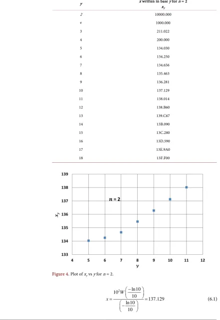
For n = 2, the solutions 𝑥𝑥 written in base y, xy shown in Table 2.

For y > 11, the xy are written using the hex notation.

There is a sharp change in the value of the xy at y = 4.

For n = 2, plot xyvs y,for5 ≤ y ≤ 11 isshown inFigure 4.

6. Connection to the Fine Structure Constant

In Equation (1.1), when n = 2 and y = 10, the equation becomes ₁₀2 ₁₀103

x

x= ×

[image:7.595.210.536.469.698.2]

and the solution is

(8)

[image:8.595.206.537.90.662.2]

DOI: 10.4236/jamp.2018.64065 732 Journal of Applied Mathematics and Physics Table 2. Solutions x in base y(xy).

y x written in base y for n = 2 _x

y

2 10000.000

e 1000.000

3 211.022

4 200.000

5 134.030

6 134.250

7 134.656

8 135.463

9 136.281

10 137.129

11 138.014

12 138.B60

13 139.C67

14 13B.090

15 13C.280

16 13D.590

17 13E.9A0

18 13F.F00

Figure 4. Plot of xy vs y for n = 2.

2 ln10

10

137.129 ln10

10

W x

−

 

 

 

= =

₋ 

 

 

[image:8.595.102.544.94.738.2]

(9)

DOI: 10.4236/jamp.2018.64065 733 Journal of Applied Mathematics and Physics The solution 137.129 is close to the inverse of the fine structure constant 137.036 [14]-[21] which is dimensionless.

The inverse of the fine structure constant α−1 is given by the expression 1 2 4π 137.036 o c e ε

α− ₌  ₌ _(6.2) where;

34

1.0545718 10− J s

= × ⋅

 , reduced Planck constant;

8 1

2.99792458 10 m s

c= × ⋅ − ,speed of light in vacuum;

12 1

0 8.854187817 10 F m

ε

₌ _× − _⋅ − _{, electric constant;} 19

1.6021766208 10 C

e= × − ,elementary charge;

1

α− _{, dimensionless constant}_[22]_.

In a recent publication Eaves [23] suggested an equation relating G and α; 2 2 2 2 exp 3 8π e q Gm

α

  ≈ _ _

  (6.3)

where;

11 3 1 2

6.67408 10 m kg s

G= × − ⋅ − ⋅ − , gravitational constant;

31

9.10938356 10 kg

e

m = × − , electron mass.

2 2 0 4 e q πε = By substituting the expression for α in Equation (6.3) we get

4

3 2 2 0 2 exp 3 32π e e

Gm c

α

ε

 

≈ _ _

 

 (6.4)

Using Equation (6.2), the Equation (6.4) becomes 4 3 2 2 2

6

1 1 64π 0

exp 1.5 e c Gm e ε α

α− _≈  − 

 

 

 _(6.5)

Substituting numerical values for the pre-exponent, 1

1 27

1.59947 10 exp

1.5

α

α− _≈ _× −  − 

 

  (6.6)

1

3.4538

1 27

1.59947 10 10

α

−      

− _≈ _× − _×  _(6.7) By taking the power of (1/289.5) on both sides of the Equation (6.8) and writ-ing the equation for α−1 yields

1 1000 1 106.6 10 α

α

−      

− _≈ _×  _(6.8) The Equation (6.8) is approximately the same as the equation 2 ₁₀3

10 10

x

x= × .

The only difference is the 102_{is 106.6 in Equation (6.8). But the Equation (6.8)}

based on the Equation (6.3) is only an approximate equation.

The value 27

1.59947 10× − in Equation (6.6) is approximately equal to the

1/1.5 , G

(10)

DOI: 10.4236/jamp.2018.64065 734 Journal of Applied Mathematics and Physics 42

3.21 10 e p

G

Gm m

c

α ₌ ₌ _× −

 (6.9)

Hence the Equation (6.7) can be written as

/

1 1 1 1.5

exp 1.5 G

α

α− _≈α  − 

 

  (6.10)

7. Conclusions

An equation in the form of n1

x y n

x y y +

       

= _{was solved graphically, numerically}

and analytically.

The plots of numerical solution x vs y indicate sharp turning points for y val-ues in-between 1 to 2.

The analytical solution was found in terms of Lambert-W function as ln

ln

n y

y W y x

y y

− 

 

 

=

₋ 

 

 

The numerical solutions can be written as x n

(

= ×0

)

yn.

The numerical solutions can also be written in base y as xy

(

n=0

)

×10n. For

(

)

5 y 0

y≥ x n= is auniversal number approximately equal to 1.37.

If n = 2 and y = 10, the solution

2 ln10

10

137.129 ln10

10

W x

−

 

 

 

= =

₋ 

 

 

(rounded) is

close to the inverse of the fine structure constant value, 137.036.

The equation ₁₀2 ₁₀103

x

x= × which gives the solution close to the fine

struc-ture constant can be derived from the equation 2 2 2

2 exp

3

8π e

q Gm

α

 

≈ _ _

  suggested

by Eaves.

The derivation resulted in an equation /

1 1 1 1.5

exp 1.5 G

α

α− _≈α  − 

 

 .

References

[1] Corless, R.M., et al. (1996) On the LambertW Function. Advances in Computation-al Mathematics, 5, 329-359. https://doi.org/10.1007/BF02124750

[2] Dence, T.P. (2013) A Brief Look into the Lambert W Function. Applied Mathemat-ics, 4, 887. https://doi.org/10.4236/am.2013.46122

[3] Kalman, D. (2001) A Generalized Logarithm for Exponential-Linear Equations. The College Mathematics Journal, 32, 2-14.

https://doi.org/10.1080/07468342.2001.11921844

(11)

Ap-DOI: 10.4236/jamp.2018.64065 735 Journal of Applied Mathematics and Physics plied Mathematics, 244, 77-89. https://doi.org/10.1016/j.cam.2012.11.021

[5] Valluri, S.R., et al. (2009) The Lambert W Function and Quantum Statistics. Journal of Mathematical Physics, 50, Article Id: 102103. https://doi.org/10.1063/1.3230482

[6] Valluri, S.R., Jeffrey, D.J. and Corless, R.M. (2000) Some Applications of the Lam-bert W Function to Physics. Canadian Journal of Physics, 78, 823-831.

[7] Scott, T.C., Mann, R. and Martinez Ii, R.E. (2006) General Relativity and Quantum Mechanics: Towards a Generalization of the Lambert W Function A Generalization of the Lambert W Function. Applicable Algebra in Engineering, Communication and Computing, 17, 41-47. https://doi.org/10.1007/s00200-006-0196-1

[8] Jain, A. and Kapoor, A. (2004) Exact Analytical Solutions of the Parameters of Real Solar Cells Using Lambert W-Function. Solar Energy Materials and Solar Cells, 81, 269-277. https://doi.org/10.1016/j.solmat.2003.11.018

[9] Goličnik, M. (2012) On the Lambert W Function and Its Utility in Biochemical Ki-netics. Biochemical Engineering Journal, 63, 116-123.

https://doi.org/10.1016/j.bej.2012.01.010

[10] Kitis, G. and Vlachos, N. (2013) General Semi-Analytical Expressions for TL, OSL and Other Luminescence Stimulation Modes Derived from the OTOR Model Using the Lambert W-Function. Radiation Measurements, 48, 47-54.

https://doi.org/10.1016/j.radmeas.2012.09.006

[11] Barry, D., et al. (1993) A Class of Exact Solutions for Richards’ Equation. Journal of Hydrology, 142, 29-46. https://doi.org/10.1016/0022-1694(93)90003-R

[12] Weisstein, E.W. (2002) Lambert W-Function.

[13] Gnanarajan, S. (2017) Solutions of the Exponential Equation yx/y_{= x or lnx/x = lny/y} and Fine Structure Constant. Journal of Applied Mathematics and Physics, 5, 386.

https://doi.org/10.4236/jamp.2017.52034

[14] Kinoshita, T. (1996) The Fine Structure Constant. Reports on Progress in Physics, 59, 1459. https://doi.org/10.1088/0034-4885/59/11/003

[15] Dirac, P.A. (1937) The Cosmological Constants. Nature, 139, 323.

https://doi.org/10.1038/139323a0

[16] Bouchendira, R., et al. (2011) New Determination of the Fine Structure Constant and Test of the Quantum Electrodynamics. Physical Review Letters, 106, Article ID: 080801.https://doi.org/10.1103/PhysRevLett.106.080801

[17] Hammer, E. (2006) Physical and Mathematical Meaning of the Alpha Constant, Einstein’s Equation, and Planck Dimensions. Industry Applications Conference, Tampa, 8-12 October 2006.https://doi.org/10.1109/IAS.2006.256848

[18] Kragh, H. (2003) Magic Number: A Partial History of the Fine-Structure Constant.

Archive for History of Exact Sciences, 57, 395-431.

[19] Sandvik, H.B., Barrow, J.D. and Magueijo, J. (2002) A Simple Cosmology with a Varying Fine Structure Constant. Physical Review Letters, 88, Article ID: 031302.

https://doi.org/10.1103/PhysRevLett.88.031302

[20] Jentschura, U.D. (2014) Fine-Structure Constant for Gravitational and Scalar Inte-ractions. Physical Review A, 90, Article ID: 022112.

https://doi.org/10.1103/PhysRevA.90.022112

[21] Jentschura, U.D. and Nándori, I. (2014) Attempts at a Determination of the Fine-Structure Constant from First Principles: A Brief Historical Overview. The European Physical Journal H, 39, 591-613.

https://doi.org/10.1140/epjh/e2014-50044-7

(12)

DOI: 10.4236/jamp.2018.64065 736 Journal of Applied Mathematics and Physics

of the Fundamental Physical Constants: 2014. Journal of Physical and Chemical Reference Data, 45, Article ID: 043102.https://doi.org/10.1063/1.4954402