Impact of Physico Chemical Properties for Soils Type Classification of OAK using different Machine Learning Techniques

Impact of Physico-Chemical Properties for Soils Type

Classification of OAK using different Machine Learning

Techniques

Himanshu Pant

Department of Computer Science and Engineering

Graphic Era Hill University Bhimtal, Uttrakhand, India

Manoj C. Lohani

Department of Computer Science and Engineering

Graphic Era Hill University Bhimtal, Uttrakhand, India

Ashutosh Bhatt

Department of Computer Science and Engineering

Birla Institute of Applied Science Bhimtal, Uttrakhand, India

ABSTRACT

Physico-Chemical properties of soils from different sites of Oak forest (Banj Oak (Quercus leucotrichophora), Kharsu Oak (Quercus semecarpifolia),Tilonj Oak(Quercus floribunda) ) in Uttarakhand are analysed. Generally, all the factors affecting this soil site that is to say sand%, silt%, clay%, available moisture%, pH value, organic matter and carbon - nitrogen ratio are analysed across three levels of soil depths (0 to 10 cm, 10 to 20 cm, 20 to 30 cm), three slopes (Hill base (HB), Hill Slope (HS) and Hill Top (HT)) and two level of disturbances (Disturbed and Undisturbed) of the Oak forest. Machine Learning algorithms can be used to forecast and automate soil site classes on different soil sample data. This Paper weighs different supervised machine learning algorithms to classify Oak forest soil site. For this classification, support vector machine (SVM), Logistic Regression (LR), Linear Discriminant Analysis (LDA), K-Nearest Neighbour (KNN), Decision Tree Classifier (CART) and Gaussian Naïve Bayes (NB) algorithms are recommended and evaluated. Simulation is run by using Python machine learning libraries. The working performance of all the algorithms observed in the form of accurateness and consistency.

Keywords

Accuracy, Classification; Oak; Physico-chemical factors; Regression; Soil Type; Support vector machines;

1.

INTRODUCTION

OAK is a deep-rooted and moderate-sized evergreen tree that belongs to the Quercus genus of the beech family and which take place in the humid and cool aspects in the lower Western Himalayan moderate forests between altitudes 1000 and 2300 m asl [1]. In Western Himalayan zone mostly researches on the physico-chemical properties of oak forest soils have dealt with the 0 to 30 cm slope depth of the forest site.

Plants are the foundation of soil organic matter, which affects the physical and chemical properties of soil such as, texture of the soil, pH values, water holding capacity and availability of the nutrients in the soil [2].

Some previous studies about physico-chemical properties of Oak forest soil were also done by researchers in various forests of Kumaun Himalaya.

The physical and chemical parameters measured from real-time field samples are the most influential features in soil characterization. Physical factors such as moisture and soil structure (soil depths and forest slopes) are correlated to the association of the particles and pores, reflecting effects on root development, speed of plant occurrence and water infiltration.

The nutrient availability, presence of other organisms and mobility of contaminants are determined by the chemical factors like pH values, organic carbon and nitrogen [3]. The soil samples of these three study sites of Oak forests (Banj Oak, Kharsu Oak,Tilonj Oak) is selected from three different depths (0–10, 10–20, 20–30 cm) using a soil auger for selected level of disturbances during rainy season and late winter, and these samples are carried out to the laboratory for analyses and examine of different physico-chemical properties.

The classes of Oak forest and use of various physical and chemical parameters necessary for soil is measured by diverse machine learning algorithms. The accuracy and predictions of various machine learning algorithms defines the best model to use for Oak forest classification.

Machine Learning is a subset of artificial intelligence. It focuses mainly on the designing the systems thereby following them to learn and make predictions based on some experience which is data in case of machines. Machine learning enables computer to act and makes data driven decision rather than being explicitly programmed to carry out the certain task. These programs are design to learn and improve over time when exposed to new data. In machine learning approaches, the algorithm is trained using labelled or unlabelled training data set to produce a model. New input data is introduced to machine learning algorithms and it make predictions based on the model. The prediction is evaluated for accuracy and if accuracy is acceptable then machine learning algorithm is deployed and if accuracy is not acceptable then machine learning algorithm is train again and again with the augmented training data set [4].

The basic idea behind the machine learning is to form supervised and unsupervised algorithms that can accept training data as an input and use statistical analysis on that training data to forecast an output while updating outputs as new data (Testing Data) becomes available.

Machine learning approach is an effective method for application in the field of analytics of data to predict the result of the system using some models and algorithms. There are numerous applications for Machine Learning (ML), the most significant of which is classification and regression [5]. In the field of agriculture, especially in soil science, classifications and regressions are performed by many supervised machine learning methods.

them on the bases of information of other, previously recognized properties. To assess the soil properties on the sample data, it is assuming that input data (Training Data) need to be divided into analogous soil groups.

In this research soil site is to stratify in the three soil depths (0-10 cm, (0-10-20 cm, and 20-30 cm), three slopes (Hill base (HB), Hill Slope (HS) and Hill Top (HT)) and two levels of disturbances (Disturbed and Undisturbed) for the Oak forest. It is suggested to improve both accurateness and consistency of the prediction and multi-class classification, soil grouping according to moisture, organic matters, pH values, sand%, silt%, clay% and carbon-nitrogen ratio. Hence, the purpose of this research is to generate the suitable classification and regression model for such approximations of the soil class to observed accuracy.

Present study is focused on the comparison of soil physico-chemical profiling of three different Oak forest types (Banj oak, Kharsu oak,Tilonj oak) of Almora region of Kumaun Himalaya, Uttarakhand.

To find the accuracy and prediction of the machine learning model, support vector machine and regression techniques are used for soil type classification based on known values of specific chemical and physical attributes in sampled profiles [6].

In this study, comparison of the performance of different classification and regression algorithms such as support vector machine (SVM), Logistic Regression (LR), Linear Discriminant Analysis (LDA), K-Nearest Neighbour (KNN), Decision Tree Classifier (Classification and Regression Tree (CART)) and Gaussian Naive Bayes (NB) are simulated using machine learning libraries in python.

The structure of this research study is as follows: In Section-2 we describe the theoretical foundations and approaches of different algorithms in classification and regression model for machine learning framework to formulate problem of Oak type categorization and approximation of the values of soil chemical and physical properties. Section-3 provides the details of experimental performance on different soil samples taken from a western Himalayan region in Almora in Uttarakhand. It section also contains the description of testing procedure and examination of the experimental results. Section-4 gives the conclusion of the paper.

2.

MATERIALS AND APPROACHES

2.1

Study area

The research study site is Almora, which is in Kumaon division, a district of Uttarakhand (India) is a scenic site situated in the lap of western Himalaya. The site Almora is located at 29.5971°N 79.6591°E and elevated from 3000 to 8450 feet above sea level. Almora has the various seasons like summer (a dry period) normally spanning from March to June, the monsoon season from July to October and winter from October to February. The average temperature of the site is 23.50C or 74.30F. The area is well populated having a population of 35513 (as of 2011 India census) and having density of 4700/km2 (1200/sq mi) with farming as a main source of action spread along the slope. The soils belong to Inceptisols, Entisols, Mollisols and Alfisols in different regions of western Himalaya [7]. In this study, the focused soil target site is the Oak forest.

2.2

Problem statement

Assume S be the collection of all the possible soil samples covering a western Himalayan area of Uttarakhand, which is represented in the form of S={x|x∈Rn} and C be the collections of L classes that relate to some primitive soil types such as Banj Oak, Kharsu Oak,Tilonj Oak.

The main objective of this paper is to find the most precise possible classification and regression using the different supervised machine learning techniques like Support Vector Machine (SVM), Logistic Regression (LR), Linear Discriminant Analysis (LDA), K-Nearest Neighbour (KNN), Decision Tree Classifier (Classification and Regression Tree (CART)) and Gaussian Naïve Bayes (NB) on given training and testing soil data set.

We compared supervised SVM algorithm to the other commonly used linear classification and regression algorithms to assess prediction accuracy and worth of the projected algorithms. The chemical and physical properties of Oak forest soil samples from depth 0-30 cm are represented in the form of measured values. The descriptions of dataset including mean, standard deviation, min and max values of the physical and chemical parameters as describe in Table-1. Mean accuracy and Standard Deviation accuracy are described in Table-2.

2.3

Classification Methodology

There are different methods for comparing machine learning algorithms to classify the sites. In Algorithms comparison, the dataset is divided in 9 attributes and 3 classes in order to show the compared accuracy result. One attribute i.e. Site is set as an output or dependent variable while the others are set as input or independent variable to the algorithms.

When we compare different machine learning algorithm for soil type classification, there should be numerous phases to be followed for the same.

i. Simulation of every algorithm is performed by using all attribute dataset and provide the accuracy of each algorithm so that we can find the best algorithms for classification.

ii. Each algorithm is re-simulated for the selection of the features by removing an attribute. This process is also known as reduced attribute or variable subset selection.

iii. Then discard the poorest class recall and to achieve the best performance of the algorithm re simulation will be done.

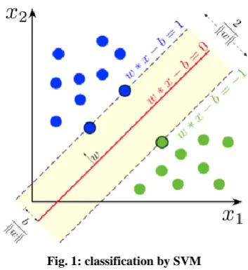
2.3.1. SVM Classification

Support Vector Machines is the kind of supervised machine learning algorithm used for classification and regression analyses. We provide labelled training data to the model for classification. Once model is prepared, it goes to testing phase. In testing phase, trained model predicts that given new data or test data belong to which class. To separate two classes in XY plane, we simply draw a centre line between two classes. This centre line is known as decision boundary or hyper plane because it is a kind of boundary in between the two classes which decides that this new data belongs to which class. This separation process of two classes is known as classification on the linearly separable data [8].

“Support Vector”. The distance of these two parallel lines from hyper plane let’s say d1 and d2. We get another distance after adding up these two distances. This new distance is known as “Margin”.

Margin=d1+d2

Margin plays a significant role to decide which hyper plane will be used. To classify data in to two classes, maximal margin hyper plane should be selected.

SVM is a universally accepted algorithm due to its simple nature. It is considered as an alternative to neural networks algorithm [9].

Fig. 1: classification by SVM

SVM (Support vector machine) is the technique to classify linearly as well as non-linear separable data [10]. Non-linear separable data is that data where we cannot separate or classify sample data by using a straight line because of misclassification. Non-linear SVM is used to classify non-linear separable data.

In Non-Linear SVM, the kernel function is used to classify non separable data. The kernel function takes the low dimensional feature space data (non separable data) as an input and gives output high dimensional feature space (separable data). There are four basic kernels functions are used to classify non-linear separable data [11]:

i. Linear kernel function ii. Polynomial kernel function iii. RBF kernel function iv. Sigmoid kernel function

In this paper, Linear Function is used as the kernel for site classification.

2.3.2 Logistic Regression

A regression analysis is used to establish a relationship between dependent variable and independent variable. We can use regression analyses most prominently where the output value or dependent variable is in numeric in nature. There are basically two types of regression:

i. Linear Regression ii. Logistic Regression

In linear regression dependent variable is in continuous in nature. It is a best choice to use linearly separable data. If we have only one independent variable with respect to dependent variable is known as simple linear regression and if we have

multiple independent variables with respect to dependent variable is known as multiple linear regressions.

Logistic regression [11] is that regression in which dependent variable is in binary form or discrete or categorical (1 for true and 0 for false) and independent variable may be either continuous or binary. The goal of the logistic regression is to find the best fitting model for independent and dependent variable relationship. Logistic regression is also called “Logit regression” [12]. Logistic regression deals with probability to measure the relationship between dependent variable and independent variable.

The main rule of logistic regression is that outcome must be either zero or one. To achieve logistic regression goal, we use S-curve or Sigmoid curve. This sigmoid function curve basically converts any value from -∞ to ∞ to discrete value which logistic regression wants or simply in binary value (0 and 1) [13]. If our data point between 0 and 1, there is a concept of threshold value. Threshold value basically indicates the probability of value either zero or one. If data point value is less then threshold value then resultant output would be zero (0) and if our data point value is greater than threshold value then resultant output would be one(1). To make this sigmoid curve, we need to make an equation.

The logistic regression equation is derived from the straight line equation [14]:

Y=C+B1X1+B2X2+…. (Range from -∞ to ∞)

In logistic equation Y can be only from 0 to 1.The final logistic equation may be written as:

log











Y

Y

1

2.3.3 Linear Discriminant Analysis

Linear Discriminant Analysis [15] is a linear model which is used to model the difference in group. This multivariate analysis that means we use more than or equal two variables to the modelling work. We build a model to separate two or more classes, objects or categories. Discriminant analysis is more like a classification technique like Logit and Probit model. Discriminant Analysis is done by comparing the means of the variable. We take several independent variables and then we see there is difference in the mean in different categories. One of the assumptions in Discriminant Analysis is that independent variables need to be continuous or normally distributed and variances of the variable should be Homogeneous.

It creates s an equation which will minimize the possibility of misclassification into their respective groups or categories. It contains the linear equation of the following form [16]:

D=a1*X1+a2*X2+……..ai*Xi+b

Where,

D = discriminant function

X= Response score for that variable A=Discriminant Coefficient B=Constant

i=No. of discriminant variable

the different group. It is very powerful classification technique validates with test data and new data but the limitation is that we cannot use categorical variable.

2.3.4 K Nearest Neighbors Classifier

K nearest neighbours [17] is a simple algorithm which uses entire data set in its training phase. Whenever prediction is required for unseen data, it searches through the entire training data set for K most similar instances and data with most similar instance is finally return as the prediction .It stores all the available cases and classifies new data or cases based on a similarity measure (e.g., distance functions). In general KNN is use in search application where we are looking in similar items. In KNN, K denotes the number of nearest neighbour which is voting class of new data or the testing data.

KNN is the supervised classification algorithms in which we have some data points which divided into different number of several categories and its tries to predict the classification of new sample from that particular population set [18]. KNN algorithm is a lazy algorithm that means it tries to only memorise the process and it does not learn itself. It classifies new data points based on similarity measure and use Euclidean distance (d) for this purpose.

d=

(

)

2

1





k

i

Xi

Yi

In k-NN classification, an object is classified to assign the most common among its k nearest neighbours (k is a positive integer, typically small). If k = 1, then the data point is simply allotted to the class of that single nearest neighbour. In KNN regression, the output is the property value for the object and which is the average of the values of k nearest neighbours.

2.3.5 Decision Tree Classifier

Decision Tree [19] is a type of classification algorithms which comes under supervised learning technique. Decision tree is the graphical representation of all the possible solution to a decision .The decision which are made is based on some condition. In the technique of classification, the role of the decision tree is as a classifier. It is like a binary tree that means it has two types of node: decision node (Test node) and leaf node. Test will be performed on the feature or attribute value. On the bases of these tests, decision will be performed. Initially entire data set is given to the root node. Depending on the result of this set, dataset would be split in the two part (D1 and D2).For particular attributes, D1 represents the all the true value and D2 represent the all the false value. This splitting process is continuing till we get leaf nodes. The significance of leaf node is that it is a classification value. The leaf nodes of the tree contain an output variable (y) which is used to make a prediction. Tree are fast to learn and very fast for making predictions.

Fig. 3. Decision Tree [19]

2.3.6 Gaussian Naïve Bayes

Naïve Bayes is a simple but powerful algorithm for predictive modelling. A naive Bayes is a classification technique based on the Bayes theorem with an assumption of independence among the predictors. It comprises of two parts which is Naïve and Bayes. In simple term Naïve Bayes classifiers assumes that the presence of the particular feature in a class is unrelated to the presence of any other feature (input variable is independent) even if this feature depends on each other or upon the existence of the other feature all of these properties independently contribute to the probability whether particular attributes belong to which class, so that it is called Naïve. Naïve Bayes is a subset of Bayesian decision theory. It’s called naive because the formulation makes some naïve assumptions. Python’s text-processing abilities which split up a document into a vector are used. This can be used to classify text. Classifies may put into human-readable form. It is a popular classification method in addition to conditional independence, over fitting, and Bayesian methods.

3.

RESULTS AND COMMENTS

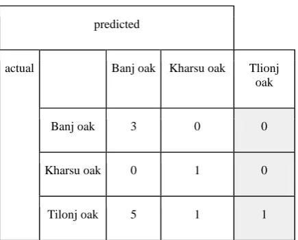
predicted

actual Banj oak Kharsu oak Tlionj oak

Banj oak 3 0 0

Kharsu oak 0 1 0

Tilonj oak 5 1 1

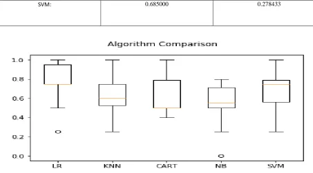
Running the list of each machine learning algorithm using python machine learning libraries with scikit-learn the mean accuracy and the standard deviation accuracy of algorithms is shown in the Table-2. The comparison of machine learning algorithm on the soil dataset of Oak forest is using a box and whisker plot [21] showing the spread of the accuracy scores across each cross validation fold for each algorithm in figure -2.

To measure the results of each machine learning algorithms, we need the multi-class confusion matrix [22]. The confusion matrix of our recognition algorithm is look like the following table:

By the confusion matrix [23], we summarize over the rows and columns. Confusion matrix shows that a given row of the matrix corresponds to specific value for the "truth", we have:

ive

FalsePosit

ve

TruePositi

ve

TruePositi

ecision





Pr

ive

FalseNegat

ve

TruePositi

ve

TruePositi

call





Re

general we can write in multiclass form: Precision (i) = Mii / ∑jMji Recall (i) = Mii / ∑jMij

The confusion matrix shows that the SVM and logistic regression has better class recall (1) and precision value is above 75%.

F1 Score are used to balance between precision and recall where there is an uneven class distribution. We can calculate F1 Score by using the formula-

call

ecision

call

ecision

F

Re

Pr

Re

*

Pr

*

2

1





The classification Report shows the precision (aka positive predictive value PPV), recall (aka sensitivity), F1-Score and support value of each type of Oak forest soil available in Himalayan region. Table -3 describe the Accuracy Score of Each machine learning algorithm apply on various physical and chemical parameters for different oak site in Himalayan Region specially in Almora district.

The simulation results of all algorithms proposed in this paper (SVM, Logistic Regression, KNN, LDA, Decision tree, Naïve Bayes) perfectly suggest that support vector machine has better accuracy for all the parameters of the soil samples for the three Oak sites in Himalayan Region.

Table 1. Soil Physico-Chemical properties of oak site

Depth(cm) Sand% Silt% Clay% Moisture% pH Value C% N% Organic

matter (%)

count 54.00 54.00 54.00 54.00 54.00 54.00 54.00 54.00 54.00

Mean 20.00 52.99 23.094 23.91 41.66 6.172 1.94074 0.169 3.541

Std 8.241 6.27 4.50 3.833 9.25 0.303 0.55 0.043 1.670

Min 10.00 6.27 15.000 16.1900 26.000 5.400 0.900 0.090 1.550

Max 30.00 66.730 34.000 32.370 63.000 6.900 3.600 0.270 13.450

Table 2. Mean and Standard Deviation of different algorithms

Algorithms Mean Accuracy standard deviation Accuracy

LR: 0.660000 0.205913

LDA: 0.735000 0.228090

KNN: 0.580000 0.215870

NB: 0.500000 0.246982

SVM: 0.685000 0.278433

Fig 2: Compare Machine Learning Algorithms

This box and whisker plot shows the comparison between different machine learning algorithms. According to this plot, it is easy to see the two mentioned algorithms (Logistic Regression and Support Vector Machine) are providing the

better accuracies. From this compared outcome, we can able to optimize the modelling process and predict the most suitable soil class for classification.

Table 3. Accuracy Score of Each algorithm

Algorithm KNN LR CART LDA NB SVM

Confusion Matrix

[[3 0 0] [0 1 0] [5 1 1]]

[[3 0 0] [0 1 0] [1 1 5]]

[[2 0 1] [0 1 0] [1 3 3]]

[[2 0 1] [0 1 0] [1 1 5]]

[[2 0 1] [0 1 0] [1 1 5]]

[[3 0 0] [0 1 0] [1 1 5]]

Classification Report

Banj Oak(s1) Precision 0.38 0.75 0.67 0.67 0.67 0.75

Recall 1.00 1.00 0.67 0.67 0.67 1.00

F1-Score 0.55 0.86 0.67 0.67 0.67 0.86

Support 3 3 3 3 3 3

Tilonj Oak(s2)

Precision 1.00 1.00 0.75 0.83 0.83 1.00

Recall 0.14 0.71 0.43 0.71 0.71 0.71

F1-Score 0.25 0.83 0.55 0.77 0.77 0.83

Support 7 7 7 7 7 7

Kharsu Oak(s3)

Precision 0.50 0.50 0.25 0.50 0.50 0.50

Recall 1.00 1.00 1.00 1.00 1.00 1.00

F1-Score 0.67 0.67 0.40 0.67 0.67 0.67

Support 1 1 1 1 1 1

4.

CONCLUSION

Soil type classification based on particular physical and chemical (Physicochemical) properties provides high levels of linearity. Different Supervised machine learning algorithms such as SVM, Logistic Regression, KNN, LDA, Decision tree, Naïve Bayes could be used to automate soil type (Oak forest soil) classification. Support Vector Machine has the best performance for classifying different types of Oak forest soil with satisfactory accuracy. This paper indicates that the physicochemical properties of the soil such as organic matters, pH values, depths of the soils, clay%, silt%, sand%, moisture% available nitrogen and carbons, are affected in cultivated (agriculture and olericulture) systems and with the help of supervised machine learning algorithms, we can easily predict the soil class and monitor the physicochemical parameters required for different Oak forest soils(Banj Oak(Quercus leucotrichophora), Kharsu Oak(Quercus semecarpifolia),Tilonj Oak(Quercus floribunda) in Himalayan area.

5.

REFERENCES

[1] Singh, J. S. and Singh, S. P., Forest vegetation of the Himalaya Bot. Rev., 1987, 52, 80–192.

[2] Johnston, A.E., 1986. Soil organic matter, effects on soil and crops. Soil Use and Management 2(3): 97-105. [3] Radhika K and Latha D. M., Machine learning model for

automation of soil texture classification, Indian J. Agric. Res., 53(1) 2019: 78-82

[4] Bishop, C. M. (2006), Pattern Recognition and Machine Learning, Springer, ISBN 978-0-387-31073-2

[5] B. Bhattacharya, D.P. Solomatine.2006. Machine learning in soil classification.Neural Networks, 19(2):186-195

[6] Kovacevic & Gajic. 2009. Soil type classification and estimation of soil properties using support vector machines, Geoderma 154 (2010) 340–347

[7] Maurya B. R., Singh V., Impact of altitudes on soil characteristics and enzymatic activities in forest and fallow lands of Almora district of central Himalaya Res. Vol. 2(1): 1-9

[8] Vapnik V.,Cortes C., Support-Vector Networks, Volume 20, Issue 3, pp 273–297 .

[9] Witten, I.H., Frank, E., 2005. Data Mining: Practical Machine Learning Tools and Techniques. 2nd ed. Elsevier, San Francisco, CA (525 pp.).

[10] C.-J. L. Chih-Wei Hsu, Chih-Chung Chang, “A Practical Guide to Support Vector Classification,” BJU Int., vol. 101, no. 1, pp. 1396–400, 2008.

[11] Kleinbaum, D.G., Kupper, L.L., Nizam, A., Muller, K.E., 2008. Logistic regression analysis. Applied Regression Analysis and Other Multivariate Methods, 4th ed. Thomson Brooks/Cole, Belmont, CA, pp. 604–634. [12] Kempen, B., Brus, D.J., Heuvelink, G.B.M., Stoorvogel,

J.J., 2009. Updating the 1:50,000 Dutch soil map using legacy soil data: a multinomial logistic regression approach. Geoderma 51, 311–326.

[13] https://machinelearningmastery.com/implement-logistic-regression-stochastic-gradient-descent-scratch-python/ [14] N.V. Boulgouris and Z.X. Chi, Gait recognition using

Radon transform and linear discriminant analysis, IEEE Transactions on Image Processing 16(3) (2007), 731–740 [15] McLachlan, G. J. (2004). Discriminant Analysis and

Statistical Pattern Recognition. Wiley Interscience. ISBN 978-0-471-69115-0. MR 1190469

[16] Garson, G. D. (2008). Discriminant function analysis. "Archived copy". Archived from the original on 2008-03-12. Retrieved 2008-03-04.

[17] Altman, N. S. (1992). "An introduction to kernel and nearest-neighbor nonparametric regression". The American Statistician. 46 (3): 175–185.

[18] D. Coomans; D.L. Massart (1982). "Alternative k-nearest neighbour rules in supervised pattern recognition : Part 1. k-Nearest neighbour classification by using alternative voting rules". Analytica Chimica Acta. 136: 15–27. doi:10.1016/S0003-2670(01)95359-0

[19] I. H. Witten, E. Frank, and M. a. Hall, Data Mining Practical Machine Learning Tools and Techniques Third Edition, vol. 277, no. Tentang Data Mining. 2011. [20] Pouria Kaviani, Mrs. Sunita Dhotre , International

Journal of Advance Engineering and Research, Volume 4, Issue 11, November -2017.

[21] McGill, Robert; Tukey, John W.; Larsen, Wayne A. (February 1978). "Variations of Box Plots". The American Statistician. 32 (1): 12–16. doi:10.2307/2683468. JSTOR 2683468.

[22] McLachlan, Geoffrey J.; Do, Kim-Anh; Ambroise, Christophe (2004). Analyzing microarray gene expression data. Wiley.