A component model for Dynamic Conditional Correlations: Disentangling interdependence from contagion

(1)

Munich Personal RePEc Archive

A component model for Dynamic

Conditional Correlations: Disentangling

interdependence from contagion

Urbina, Jilber

Department of Economics, Universitat Rovira i Virgili (URV),

Centre de Recerca en Economia Industrial i Economia Pública

(CREIP), Banco Central de Nicaragua (BCN)

12 September 2013

Online at

https://mpra.ub.uni-muenchen.de/75579/

(2)

A Component Model for Dynamic Conditional

Correlations: Disentangling Interdependence from

Contagion

Jilber Urbina

∗

Abstract

We analyze whether the crisis sourced in US is spread over the world by contagion

or through interdependence. Within this work, contagion is defined as a significant

increase in cross-correlations after a crisis hits a country, we assumed that correlations

are not constant over time and also evolve according to a GARCH(1,1)-type structure

which give rise to the use of the popular DCC model introduced by Engle (2002) and

extended in Colacito et al. (2011) to disentangle the short and long run component of

the total correlation of the portfolio under study. We link interdependence with long-run

fluctuations in correlations and contagion is associated with the short-run correlations.

JEL codes: C01, C58, G01, G15.

Keywords: contagion, financial crisis, stock markets, global transmission, market integration,

Dy-namic Conditional Correlations.

∗_{This paper was totally developed at the Department of Economics, Universitat Rovira i Virgili and}

(3)

1 Introduction

Assessment of the transmission mechanisms of financial crisis across countries based on

cor-relations have been payed a lot of attention since King and Wadhwani (1990) and then

reinforced by Forbes and Rigobon (2002). Correlation approach is useful since it provides a

straightforward way to test for contagion (see Forbes and Rigobon, 2002), nevertheless the

“static” correlation approach is very simplistic, it splits the sample into two subsamples

(pre-crisis and post-(pre-crisis periods) and performs a test of significant increase in correlations over

these two periods where the underlying correlations are fixed within periods, none dynamic

is involved in the correlations.

The lack of temporal dynamics in the correlations can be overcome by using a Dynamic

Conditional Correlation (DCC) model, first introduced by Engle (2002). Several attempts

have been done to test for contagion by averaging the dynamic correlations belonging to

each subsamples and then performing a classical t-test for mean differences, see for instance

Wang and Nguyen Thi (2013), Naoui et al. (2010a), Naoui et al. (2010b) and Chiang et al.

(2007) . These works rely on defining contagion as an increase in cross-market linkages after

a exogenous negative shock in one country or group of countries (such definition corresponds

to the World Bank’s “very restrictive” definition), but none of them show the time varying

behavior of both interdependence and contagion.

We try to shed some light on the gap, which in terms of Rigobon (2003), no satisfactory

procedure has been developed to be able to answer the question whether contagion occurs

or not using the correlation-based definition since the seminal contribution by King and

Wadhwani (1990).

We use a component model for the DCC to capture both, interdependence and contagion

via a parsimonious parameter structure and still rely on thevery restrictive definition of

con-tagion, but allowing the correlations to be time varying. Using the DCC-MIDAS1 _introduced

by Colacito et al. (2011) we can disentangle both, the long run and short run components

of the time varying correlations which can allows us to associate the former with contagion

1

DCC-MIDAS: Dynamic Conditional Correlation - Mixed Data Sampling Model.

(4)

and the latter with interdependence.

Within this framework we identify interdependence which is in itself a contribution since

it helps to better understand contagion. Forbes and Rigobon (2002) discussed the influence

of heteroscedasticity over the correlations and furthermore, a correction is also proposed.

Nevertheless, the test over the corrected correlation operates in a static environment such

that contagion can be wrongly diagnosed, mainly because interdependence effects have not

been discounted from the correlations.

As discussed inForbes and Rigobon(2002) correlation after a negative shock can increase

because of heteroscedasticity, however, as markets moves more and more together due to

market integration, it is plausible to think that interdependence also varies over time and

moves in the same direction of market integration, therefore, correlations also can be increased

by the effect of integration and such integration is represented by interdependence which is

not explicitly taken into account in previous works.

The above ideas are relevant since financial links play an important role in economic

integration of an individual country into the world market (Dornbusch et al., 2000), this

means that a financial crisis in one country can lead to direct financial effects to other

countries. In line with Dornbusch et al. (2000) the spread of a financial crisis depends

primarily on the investors’ behavior and on the degree of financial market integration, they

claims that in this sense, financial markets facilitate the transmission of real or common

shocks but do not cause them. As these kind of links (financial and trade) give rise to market

integration (interdependence) play and important role for transmitting crisis, a measure of

such links over time become crucially important, this measure is provided in this context by

the long-run correlation given by the MIDAS filter.

Long-run component can be seen as the measure of financial market integration which is

plausible to be modeled as a slowly moving average of correlations due to the fact that such

integrations are neither constant overtime nor fast-moving, it evolves slowly.

Empirical works on contagion has been focused mainly on the co-movements in asset

prices rather than on “excessive” co-movements among them (Dornbusch et al., 2000). We

(5)

of interdependence, this is done by subtracting from the short-run correlation at time t,

the corresponding long-run correlation. Once we have the correlation without the effects of

interdependence, we can perform a test for contagion.

In order to estimate both kind of correlation, we use recently introduced DCC-MIDAS

model of Colacito et al. (2011). DCC-MIDAS model is not a new model since is was

intro-duced by Colacito et al.(2011), nevertheless the novelty of our approach is the application of

this model to the context of contagion vs interdependence, where we associate contagion to

short-lived events (short run correlations) and interdependence is directly linked to long-run

correlations.

After adjusting the correlations by discounting the interdependence effects we perform a

test for contagion leading to the conclusion that the Global Financial Crisis triggered in US

was spread to other countries through interdependence. We only find evidence of contagion

for one pair of countries: Brazil - Japan.

The remaining of this work is arranged as follows: insection 2 we present the model, its

notation, the estimation procedure and the hypothesis test strategy. Empirical application

is developed in section 3, some concluding remarks are in section 4.

2 Model Specification

2.1 Notation and Preliminaries

We begin this section by providing the meaning of the notation used throughout this work.

Letrt = [r1_,t, . . . , r_n,t]′ be a vector of returns such that follows the processr_t ∼N(µ,H_t)

with:

H_t=D_tQ_tD_t, (1)

where µ is the vector of unconditional means, Ht is the conditional covariance matrix, Qt

is the conditional correlation matrix and Dt is a diagonal matrix with conditional standard

deviations on the diagonal, with:

(6)

Qt=E[ξtξt′ |Ωt−1] (2)

ξt=D−

1

t (rt−µ), (3)

where ξt is a vector of standardized residuals andΩt−1 is the information set available up to

t₋1. Therefore, we can write the vector of returns as rt=µ+H

1_/2

t ξt with ξt∼N(0,In)

2.2 The DCC–MIDAS model

The DCC-MIDAS model is a natural extension to DCC model, they both are very similar in

their formulation and the main difference between them is that DCC-MIDAS has two

com-ponents: a long-run and a short-run component for correlations. The standard formulation

of a DCC models is shown in (4) and the one corresponding to a DCC-MIDAS model is (5),

one can tell that the difference between them is the construction of R¯. For the standard DCC model R¯ represents the matrix of unconditional correlations which is time invariant, in contrast for the DCC-MIDAS,Rbecomes intoR¯t(ω), which is time varying and its behaviour is entirely determine by a slowly moving average weighting, ω. R¯t(ω) is interpreted as the long-run component and its counterpart, the short-run component, is left to be represented

by Qt:

Qt= (1−a−b)R¯ +aξ_t₋1ξ_t′₋1+bQt₋1 (4)

Qt = (1−a−b)R¯t(ω) +aξ_t₋1ξ′_t₋1+bQt₋1 (5)

where the long-run component is R¯t(ω) = PK

l=1Φl(ω)⊙Ct₋1 a slowly moving average of

some correlation matrix denoted by Ct₋l with typical element being c_i,j,t₋l. The operator

⊙ denotes the Hadamard product. For the short-run component to be a correlation, the following transformation is needed Qt∗ = {diag(Qt)−

1

Qtdiag(Qt)−

1

} (Engle, 2002), where

q∗

(7)

If we denote the typical element ofQt as q_i,j,t and if the typical element of matrix R¯t is

denoted by ρ¯i,j,t, then we can write the full formulation of the DCC-MIDAS as follows:

qi,j,t= (1−a−b)¯ρi,j,t+aξi,t−1ξ_j,t₋1+bq_i,j,t₋1 (6)

q∗

i,j,t=

q_i,j,t

√_q i,i,tqj,j,t

¯

ρi,j,t= K

X

l=1

ϕ(ω)ci,j,t−l

c_i,j,t₋_l=

Pt−l

k=_t₋_l₋_N ξi,kξj,k

qPt−l k=_t₋_l₋_Nξ

2

i,k

qPt−l k=_t₋_l₋_Nξ

2

j,k

ϕ(ω) = 1−

1

K

ω−1

K

P

j=1

1₋ _Kjω−1

According to the formulation of system (6), the value of N is needed for estimating

the weighted correlation ci,j,t−l which only accounts for the last N past observations in its

calculation, then over these correlations, a long run correlation is estimated as a weighting

average of all the K past values giving weights ϕ(ω).

Under this formulationq∗

i,j,t is the short run correlation between assets i and j, whereas

¯

ρi,j,tis a slowly movinglong runcorrelation. Furthermore,ϕ(ω)are the so called Beta weights

which governs the movements of the long run component, this weighting scheme allows us

to extract the slowly moving secular component around which the short-run component

evolves. Lag lengths are denoted by N and span lengths of historical correlations are left to

be represented by K, we consider N and K are constant for all assets.

Rewriting the first equation of system (6) as:

q_i,j,t₋ρ¯_i,j,t =a(ξ_i,t₋1ξ_j,t₋1 −ρ¯_i,j,t) +b(q_i,j,t₋1−ρ¯_i,j,t), (7)

conveys de idea of short run fluctuations around a time-varying long run relationship.

(8)

2.3 Estimation procedure

The estimation procedure is fully described in Colacito et al. (2011), here we briefly point

out the main aspects. In order to estimate the parameters of the DCC-MIDAS model we

follow the two step procedure of Engle (2002). Let ψ2 _{be the collection of parameters of the}

univariate GARCH model and let Ξ be the vector of DCC parameter (a, b, ω), the

quasi-maximum likelihood (QL) takes the following form:

QL(ψ,Ξ) =QL1(ψ) +QL2(ψ,Ξ) (8)

=₋

T

X

t=1

(nlog(2π) + 2log_|D_t|+r′

tD

2

trt)− T

X

t=1

(log_|R_t|+ξ′

tR−

1

t ξt+ξt′ξt).

The separation of QL(ψ,Ξ) into QL1(ψ) and QL2(ψ,Ξ) indicates that we can first

esti-mate the parameters of the univariate GARCH-type processes contained in ψ by maximizing

QL1(ψ) to obtain ψˆ, then we can plug ψˆ in QL2(ψ,Ξ) so that it becomes into QL2( ˆψ,Ξ)

where standardized residuals ξˆ= ˆD−1

t (rt−µˆ) are used in the second stage.

System (6) requires setting two extra parameters: N the MIDAS lag length and K, the

span lengths of historical correlations, both are chosen from the parameter space by maximum

likelihood profiling. The profiling procedure of the likelihood function is performed over the

maximization of QL2(ψ,Ξ), once we get the “optimal” N and K we reestimate the entire

model using the complete likelihood defined by

log_L =₋1 2

T

X

t=1

(nlog(2π) + 2 log_|Dt|+r′tD−

1

t D−

1

t rt−ξt′ξt+ log|Rt|+ξt′R−

1

t ξt), (9)

maximizing it in one step to obtain the relevant standard errors of the estimated coefficients

to perform individual hypothesis tests.

2

(9)

2.4 Testing procedure

In this section we present the strategies to test for contagion based on the dynamic

correla-tions estimated under the DCC-MIDAS scheme.

One of the alternatives consist of testing H0 : a = 0 which implies that under the null,

qi,j,t is determined by (1−b)ρi,j,t(ω) +bi,j,t−1 with0≤b <1. If the empirical evidence do not

reject the null, then interdependence can be reached as the conclusion of the test. However,

if H0 :a = 0 turns out to be rejected, then this constitutes contagion defined as in Corsetti

et al.(2005) who consider that “for contagion to occur, the observed pattern of comovements

in asset prices must be too strong (or too weak) relative to what can be predicted conditional

on a constant mechanism of international transmission".

Corsetti et al. (2005) definition conveys the idea that contagion can be assessed through

performing a test for increases or decreases in the conditional correlations, in our context this

boils out to be a test overH0 :a= 0 to determine whether the co-movements are too strong

or too weak, this is the reason why the one-step estimation of the DCC-MIDAS is required.

Another approach to test for contagion is using directly the time-varying conditional

correlations produced by the model. Considering contagion as an increase in the mean

correlation after a crisis, if such increase stemmed from a model which acts like a filter

discounting the economic fundamentals, then it is plausible to assume that the increase

(positive excess) in correlations is due to irrational reactions of the agents in the markets. A

way to measure this excess based on the daily conditional time-varying correlation from the

DCC-MIDAS model is:

ql∗

i,j =

1

Tl

X

t

q∗

i,j,t−ρi,j,t(ω)

✶(t _∈precrisis) (10)

qh∗

i,j =

1

Th

X

t

q∗

i,j,t−ρi,j,t(ω)

✶(t_∈crisis) (11)

where ✶(_·) is an indicator function that takes value 1 when condition in () is met and 0

otherwise. Tl = ✶P_t(t_∈precrisis) is the sample size corresponding to the stable period,

(10)

The proposed test of contagion interprets an increase in mean excess of correlations as

evidence of contagion because it represents additional comovements in asset returns during

the crisis period not present in the precrisis period. As contagion represents the additional

comovements in asset returns over that predicted by changes in the market fundamentals, the

identification of contagion requires the extraction of market fundamentals from the returns

series (Fry et al., 2010). Within the DCC-MIDAS approach here proposed, we associate

market fundamentals with the long-run correlations mainly because the MIDAS part filters

the series and the result can be used as a proxy for the fundamentals, leading to identification

of contagion as any excess of short-run correlation from the levels of long-run correlations.

As a consequence the hypothesis test boils out to be as follows:

H0 : qh_i,j∗ ≤ql_i,j∗ (12)

H1 : qh_i,j∗ > ql_i,j∗ (13)

which is a traditional mean difference based on the standard t-test as that of Naoui et al.

(2010b). For that we use:

c

ql∗

i,j = 1 Tl X t d q∗

i,j,t−ρi,j,t(ωb)

✶(t_∈precrisis) (14)

c

qh∗

i,j = 1 Th X t d q∗

i,j,t−ρi,j,t(ωb)

✶(t _∈crisis) (15)

where qd∗

i,j,t and bω are obtained from the MLE of the DCC-MIDAS model.

Another alternative to test for contagion is using Corsetti et al. (2005) definition and to

test whether contagion occurs by setting a threshold (τ). Testing whether deviation of the

short-run correlation from the long-run correlation is bigger (smaller) than τ is in line with

the idea that the comovements should be too strong (or too weak) for contagion to exist. In

this case, the hypothesis test can be written as follows

H0 :

q∗

i,j,t−ρi,j,t(ω)

_≤τ (16)

H1 :

q∗

i,j,t−ρi,j,t(ω)

> τ (17)

where H0 implies interdependence and H1 contagion. Usually τ is proportional to the

stan-dard deviation of q∗

i,j,t−ρi,j,t(ω)

(11)

3 Empirical application

One of the tests of contagion presented in the previous section is now applied to identify

potential contagious linkages from the US stock market to other stock markets during the

subprime mortgage crisis. Our analyzed period goes from January 1, 2004 to December 31,

2012. Stock indexes and countries chosen for the analysis are in ??.

First, we estimate the short and long run correlation of asset returns. As we pointed out

before, we address the problem of selecting MIDAS lags by following Colacito et al. (2011)

and Engle et al.(2006), we compare different DCC-MIDAS models with different time spans

via profiling of the likelihood function.3

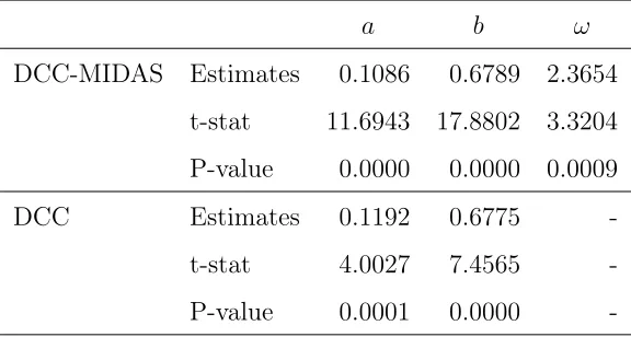
InTable 1we report the coefficients of the DCC-MIDAS and also the resulting estimates

of a DCC. Our estimation is somehow restrictive because we only consider one parameter

(ω) to account for the long run dynamics. For the short run dynamics we use DCC of order

(1,1), which means only one a and one b.

Results inTable 1 show that DCC-MIDAS parameters are very close to the DCC

param-eters as is recurrent feature inEngle et al. (2006), the superiority of DCC-MIDAS over DCC

is the capability of disentangling the short run from the long run correlation which permits

analyzing the behavior of them simultaneously.

Time varying correlations based on the DCC-MIDAS scheme are plotted on Figure 1,

Figure 2 and Figure 3, the black lines in each plot represents the short run correlation

meanwhile the long run correlation is shown in red, the dashed line splits the entire sample

into two subsamples: precrisis period and crisis period as it is conventionally done in the

contagion literature based on correlation. A visual analysis of these figures suggests no

relevant changes in the linkages between countries neither in the general short run correlation

behavior nor in the long run, from this fact we can derive the cautious “conclusion" that the

economies exhibits strong linkages in all states of the world, this situation can be interpreted

as interdependence, nevertheless, in order to formally draw any conclusion about the absence

of contagion during the analyzed period, we perform a statistical hypothesis testing.

3

See details of the procedure in Engle et al.(2006).

(12)

[image:12.612.162.450.131.285.2]

Table 1: DCC MIDAS and DCC results.

a b ω

DCC-MIDAS Estimates 0.1086 0.6789 2.3654

t-stat 11.6943 17.8802 3.3204

P-value 0.0000 0.0000 0.0009

DCC Estimates 0.1192 0.6775

-t-stat 4.0027 7.4565

-P-value 0.0001 0.0000

-Note: The top panel reports the estimates of the DCC-MIDAS while the

bottom panel shows the DCC estimates. We setK=_N = 528 as suggested by the likelihood profiling.

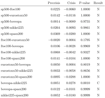
Table 2consists of all the possible combinations of pairwise correlations for the analyzed

sample, since we have 6 countries (stock markets) then we can compute 15 q¯l_i,j,t andq¯_i,j,th and

perform the test specified in subsection 2.4. Hypothesis test suggests no contagion for all

pair of countries except for Brazil and Japan where the p-value confirm the rejection of the

null even at 1% significance level.

The results of the test confirm that transmission of the crisis was due to real linkages,

(13)

[image:13.612.136.480.206.530.2]

Table 2: Contagion test results.

Precrisis Crisis P-value Result

sp500-ftse100 0_.0225 ₋0_.0060 1_.0000 _N

sp500-eurostoxx50 0_.0142 ₋0_.0116 1_.0000 _N

sp500-bovespa 0_.0014 ₋0_.0089 0_.9755 _N

sp500-nikkei225 0_.0264 0_.0093 0_.9861 _N

sp500-spasx200 0_.0369 ₋0_.0200 1_.0000 _N

ftse100-eurostoxx50 ₋0_.0020 0_.0004 0_.1795 _N

ftse100-bovespa 0_.0106 ₋0_.0028 0_.9969 _N

ftse100-nikkei225 0_.0068 ₋0_.0042 0_.9327 _N

ftse100-spasx200 0_.0141 ₋0_.0104 1_.0000 _N

eurostoxx50-bovespa 0_.0050 0_.0004 0_.8019 _N

eurostoxx50-nikkei225 0_.0033 ₋0_.0058 0_.8656 _N

eurostoxx50-spasx200 0_.0095 ₋0_.0288 1_.0000 _N

bovespa-nikkei225 0_.0051 0_.0278 0_.0010 _C

bovespa-spasx200 0_.0122 ₋0_.0101 0_.9999 _N

nikkei225-spasx200 0_.0052 ₋0_.0180 0_.9999 _N

footnotesizeNote: column 1 indicates the pairs of countries for which

cor-relation is computed, columns 2 and 3 have the mean of those corcor-relations,

column 4 holds the p values associated to the test and the last column

contains anN _{when No-contagion and it has a}C _{when there is empirical}

evidence of contagion.

(14)

0 200 400 600 800 1000 1200 −1.0 −0.5 0.0 0.5 1.0

Dynamic Conditional Correlations

Short run correlations Long run correlations

DCC MIDAS SP500 − FTSE100

0 200 400 600 800 1000 1200 −1.0

−0.5 0.0 0.5 1.0

DCC MIDAS SP500 − EUROSTOXX50

0 200 400 600 800 1000 1200 −1.0

−0.5 0.0 0.5 1.0

DCC MIDAS SP500 − BOVESPA

0 200 400 600 800 1000 1200 −1.0

−0.5 0.0 0.5 1.0

DCC MIDAS SP500 − NIKKEI225

0 200 400 600 800 1000 1200 −1.0

−0.5 0.0 0.5 1.0

[image:14.612.117.484.196.568.2]

DCC MIDAS SP500 − SPASX200

(15)

0 200 400 600 800 1000 1200 −1.0 −0.5 0.0 0.5 1.0

DCC MIDAS FTSE100 − EUROSTOXX50

0 200 400 600 800 1000 1200 −1.0

−0.5 0.0 0.5 1.0

DCC MIDAS FTSE100 − BOVESPA

0 200 400 600 800 1000 1200 −1.0

−0.5 0.0 0.5 1.0

DCC MIDAS FTSE100 − NIKKEI225

0 200 400 600 800 1000 1200 −1.0

−0.5 0.0 0.5 1.0

DCC MIDAS FTSE100 − SPASX200

0 200 400 600 800 1000 1200 −1.0

−0.5 0.0 0.5 1.0

DCC MIDAS EUROSTOXX50 − BOVESPA

0 200 400 600 800 1000 1200 −1.0

−0.5 0.0 0.5 1.0

[image:15.612.84.652.112.466.2]

DCC MIDAS EUROSTOXX50 − NIKKEI225

Figure 2: Long and short correlations for returns.

(16)

0 200 400 600 800 1000 1200 −1.0

−0.5 0.0 0.5 1.0

DCC MIDAS EUROSTOXX50 − SPASX200

0 200 400 600 800 1000 1200 −1.0

−0.5 0.0 0.5 1.0

DCC MIDAS BOVESPA − NIKKEI225

0 200 400 600 800 1000 1200 −1.0

−0.5 0.0 0.5 1.0

DCC MIDAS BOVESPA − SPASX200

0 200 400 600 800 1000 1200 −1.0

−0.5 0.0 0.5 1.0

[image:16.612.115.490.107.488.2]

DCC MIDAS NIKKEI225 − SPASX200

Figure 3: Long and short correlations for returns.

4 Conclusions

In this paper we analyzed whether the crisis sourced in US is spread over the world by

contagion or just through real linkages known as interdependence. Within this chapter,

contagion is defined as a significant increase in cross-correlations after a crisis hits a country,

we assumed that correlations are not constant over time and also assuming that they evolves

according to a GARCH(1,1)-type structure which give rise to the use of the popular DCC

(17)

run and long run component of the total correlation of the portfolio under study.

Our results suggest that linkages between stock markets remains the same before and after

the crisis, there is no evidence of significant increase in correlations, therefore interdependence

is the main channel of transmission of the crisis which is plausible since stock markets are more

and more integrated and the lagged values of the correlation associated to the interdependence

are dominant over the influence of the short run correlations.

Evidence of contagion is only found for Brazil and Japan. It is worthy to say that the

test only identifies the existence/non-existence of contagion but it is not allow to identify the

directionality of such a contagion, for the case of Brazil and Japan we found the correlation

strengthened after the crisis in US providing evidence of contagion but we do not know if

contagion ran from Brazil to Japan or in the other way around.

(18)

References

Chiang, T. C., Jeon, B. N., and Li, H. (2007). Dynamic correlation analysis of financial

contagion: Evidence from Asian markets. Journal of International Money and Finance,

26(7):1206–1228.

Colacito, R., Engle, R. F., and Ghysels, E. (2011). A component model for dynamic

corre-lations. Journal of Econometrics, 164(1):45–59.

Corsetti, G., Pericoli, M., and Sbracia, M. (2005). Some contagion, some interdependence?:

More pitfalls in tests of financial contagion. Journal of International Money and Finance,

24(8):1177 – 1199.

Dornbusch, R., Park, Y. C., and Claessens, S. (2000). Contagion: Understanding How It

Spreads. World Bank Research Observer, 15(2):177–97.

Engle, R. (2002). Dynamic Conditional Correlation: A Simple Class of Multivariate

Gen-eralized Autoregressive Conditional Heteroskedasticity Models. Journal of Business &

Economic Statistics, 20(3):339–350.

Engle, R., Gysels, E., and Sohn, B. (2006). On the economic sources of stock market volatility.

NYU and UNC unpublised manuscript.

Forbes, K. and Rigobon, R. (2002). No Contagion, Only Interdependence: Measuring Stock

Market Comovements. The Journal of Finance, 57(5):2223–2261.

Fry, R., Martin, V. L., and Tang, C. (2010). A new class of tests of contagion with

applica-tions. Journal of Business & Economic Statistics, 28(3):423–437.

King, M. A. and Wadhwani, S. (1990). Transmission of Volatility between Stock Markets.

The Review of Financial Studies, 3(1):5–33.

Naoui, K., Khemiri, S., and Liouane, N. (2010a). Crises and Financial Contagion: The

(19)

Naoui, K., Liouane, N., and Brahim, S. (2010b). A Dynamic Conditional Correlation Analysis

of Financial Contagion: The Case of the Subprime Credit Crisis. International Journal of

Economics and Finance, 2(3):85–96.

Rigobon, R. (2003). On the measurement of the international propagation of shocks: is the

transmission stable? Journal of International Economics, 61(2):261 – 283.

Wang, K.-M. and Nguyen Thi, T.-B. (2013). Did China avoid the Asian flu? The contagion

effect test with dynamic correlation coefficients. Quantitative Finance, 13(3):471–481.