A COMPUTATIONAL AND BEHAVIOURAL STUDY
Fraser Aitken
A Thesis Submitted for the Degree of PhD
at the
University of St Andrews
2019
Full metadata for this item is available in
St Andrews Research Repository
at:
http://research-repository.st-andrews.ac.uk/
Please use this identifier to cite or link to this item:
http://hdl.handle.net/10023/19158
Testing the Predictive Coding Account of Temporal Integration in the Human
Visual System-A Computational and Behavioural Study
Fraser Aitken
A Thesis Submitted for the Degree of PhD at the University of St Andrews
October 2019
All data for this item is available in the St Andrews Research Repository at
This work was supported by the University of St Andrews Wellcome trust strategic support grant [grant code APSC-ISSFFA].
Research Data/Digital Outputs access statement
Research data underpinning this thesis are available at https://osf.io/dashboard & http://research-repository.st-andrews.ac.uk/
Candidate's declaration
I, Fraser Aitken, do hereby certify that this thesis, submitted for the degree of PhD, which is approximately 68,000 words in length, has been written by me, and that it is the record of work carried out by me, or principally by myself in collaboration with others as acknowledged, and that it has not been submitted in any previous application for any degree.
I was admitted as a research student at the University of St Andrews in September 2015.
I received funding from an organisation or institution and have acknowledged the funder(s) in the full text of my thesis.
Date Signature of candidate
Supervisor's declaration
I hereby certify that the candidate has fulfilled the conditions of the Resolution and Regulations appropriate for the degree of PhD in the University of St Andrews and that the candidate is qualified to submit this thesis in application for that degree.
Date Signature of supervisor
Permission for publication
library or research worker, that this thesis will be electronically accessible for personal or research use and that the library has the right to migrate this thesis into new electronic forms as required to ensure continued access to the thesis.
I, Fraser Aitken, confirm that my thesis does not contain any third-party material that requires copyright clearance.
The following is an agreed request by candidate and supervisor regarding the publication of this thesis:
Printed copy
No embargo on print copy.
Electronic copy
No embargo on electronic copy.
Date Signature of candidate
A major goal of vision science is to understand how the visual system maintains behaviourally relevant perceptions given the level of uncertainty in the signals it receives. One proposed solution is that the visual system applies predictive coding to its inputs based on the integration of prior
knowledge and current stimulus features. However, support for some vital aspects of predictive coding in the temporal domain is lacking and simpler accounts of temporal integration also exist. The aim of this thesis was to test two key attributes of predictive coding in time a) does the visual system apply adaptive weighting to prediction errors and b) can the visual system apply probalistic
information learnt from stimulus sequences when making predictions. In chapters 3 & 4, we tested predictive coding’s ideas of how prediction errors are weighted under the theoretical guidance of a temporal integration model linked to predictive processing, called the Kalman filter. Here, both experiments supported predictive coding. We showed that, consistent with the Kalman filter, visual estimates and the way estimation errors were corrected, adapted to stimulus behaviour and viewing conditions. In chapter 5, we assessed the ability of the visual system to integrate conditional relationships present in sequences of stimuli when making predictions. To do this, we inserted a stimulus sequence that changed and omitted trials based on Markov transition probabilities that made some transitions more or less probable and assessed reaction times and omission trial responses. Reaction time data was consistent with predictive coding, in that more predictable changes elicited faster responses. Omission trials data, was though, less clear. When faced with no stimulus,
I would first like to thank my supervisor Dr Justin Ales for his guidance and support throughout my PhD. I will be forever grateful to him for providing the opportunity to study at such a fabulous University and extend this gratitude to the Wellcome trust strategic fund for providing financial support. An unforgettable experience. The end of this PhD marks the end of 8 years as a student at one level or another. With this in mind, I would like to thank Alan Searle at the University of Hull for making me believe that I could progress in academia and Professor Alex Wade at the University of York for inspiring my interest in the visual system. I would also like to thank everyone in the Vision group at St Andrews, in particular Andy Mackenzie for his words of wisdom about negotiating a PhD. Pastorally, I would also like to extend thanks to Professor Julie Harris and Dr Ines Jentzsch for their chats and guidance during my time at St Andrews. Always happy to listen to students and provide useful advice when required. Of course, no acknowledgements list would be complete without mentioning the good folk of the Lilac room. Big thanks go to my friends Abigail and Alex, who have been ‘in it’ from the beginning with me since I arrived at St Andrews. No mention of the Lilac room would be complete without mentioning Alonso, Sonny, Gierdre, Jenny and especially Bashar and ‘Charley’ Charles Ogunbode for their dependable good humour and friendship. No doubt the
Abstract………IV Acknowledgements………...…...V
Chapter 1 Vision and uncertainty-how to deal with a dynamic and noisy world………1
1. General introduction ...1
1.1 Vision-a vital behavioural tool ……….…..1
1.2 The central problem for vision……….……..1
1.3 Uncertainty in visual information-Variability in visual inputs………..…2
1.4 Sources of variability in visual information………...…3
1.5 External variability……….4
1.6 Internal variability. ………. ……….….7
1.7 Variability in signals and measurements produces little effect on perception and behaviour-Application of prior knowledge……….……...…….11
1.8 Types of temporal regularity……….…...10
1.9 Broad evidence that the visual system integrates temporal structure when interpreting variable retinal measurements………...11
1.10 Two predictive integration strategies- Assume stability and predict based on the average of values observed over time or learn the conditional relationships between stimuli and predict…...…..13
1.11 Perceptual averaging and perceptual inference………....………...14
1.12 Predictive coding account of temporal integration-basic ideas……….……16
1.13 Rao and Ballard (1999) predictive coding in sensory cortex model…………....……….….17
1.14 Missing pieces of the predictive coding puzzle-Temporal predictive coding model and explicit perceptual averaging model………...18
1.15 Lack of specific computational temporal models make the behavioural signatures of fixed weighted perceptual averaging and predictive coding difficult to identify in current literature……....20
1.19 Research questions and flow of experimental chapters
List of figures chapter 1
Fig 1 Illustration of the position of the isolated occipital cortex at the posterior of the brain source of
signals and the internal structure of the retina which provides visual information to the cortex………2
Fig 2 The general relationship between variability and uncertainty………3
Fig 3 Nosie and poor weather………..……5
Fig 4 Effects of reduced light on retinal measurements………..……….……6
Fig 5 Variability and stimulus information………..8
Fig 6 Schematic illustration of Rao & Ballard’s (1999) predictive coding model………….………...18
Fig 7 Fischer & Whitney’s (2104) experimental design and task……….22
List of tables Table 1-Predictive coding vs fixed rate perceptual averaging………...………20
Chapter 2 The Kalman filter and fixed weighted average models- Concepts, math and motivations………....31
2.1 Weighted average model. Concepts, assumptions and example...31
2.2 The Kalman Filter-aims, concepts and example... 34
2.3 Equations...………..… 42
2.3.1 Fixed weighted average model equations...43
2.3.2. Kalman Filter... ...43-46 List of important equations Equations 2, 3 & 4 Fixed weighted average model………...42
Equation 6 General Kalman filter estimation equation ………… ……….…….43
Equation 7 Kalman gain……….44
Figure 1 How a fixed weighted average makes estimates of fluctuating voltage values………...……34
Figure 2 Example of the distinction between proximal and distal variance………..………..…..40
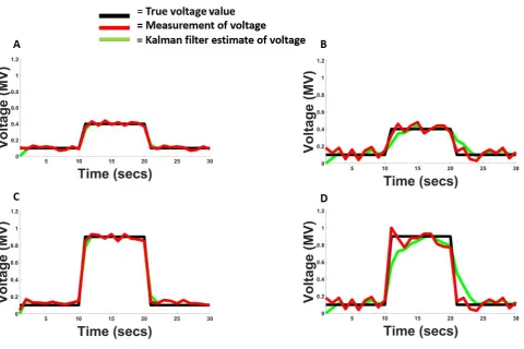
Figure 3 How a Kalman filter makes estimates of fluctuating voltage values………..………..….…41
Chapter 3 Serial dependence in visual estimates explained within a predictive coding framework……….49
3.1 Abstract……….………...………49
3.2 Introduction………...54
3.3 Methods………..………..54
3.7.3 Proximal variance calibration experiment………54
3.3.1 Main experiment one- Testing serial dependence under high distal variance versus low and high proximal variance………..57
3.3.2 Experiment two-Testing serial dependence under low distal variance versus low and high proximal variance………...58
3.4 Analyses and statistical tests………...……59
3.5 Results………...….. 62
3.5.1 Proximal variance calibration……….….…… 62
3.5.2 Main experiment one……….….. 63
3.5.2 Main experiment two……….………....……….… 72
3.6 Supplemental experiment……….……….……..81
3.6.1 Methods...82
3.6.2. Analyses...83
3.6.3 Results...83
3.7 Discussion and conclusion ………...……87
List of figures Figure 1 Proximal variance calibration experimental design and procedure…………..………...……56
Figure 4-Group level differences in proximal variance obtained during our proximal variance …...63
Figure 5 Estimated and model fitted Kalman gains for experiment one……… ………....…64
Figure 6 Mean model fitted weights for experiment one………..…….65
Figure 7 Four individual serial dependence plots for four individual participants………..…..68
Figure 8 Group serial dependence plot (experiment one)………..……70
Figure 9 Mean n back regression slopes for experiment one………..…….…..71
Figure 10 Estimated and model fitted Kalman gains for experiment two……….………. 73
Figure 11 Mean model fitted weights for experiment two……….………74
Figure 12 Four individual serial dependence plots for four individual participants in the 5% contrast condition………...…77
Figure 13 Group serial dependence plot………....…....79
Figure 14 Serial dependence magnitude towards trial presented 1-6 trials back………....…...80
Figure 15 Design and task for the supplemental serial dependency experiment…………..……….…84
Figure 16 Modelled Kalman gains supplemental experiment………...…….…...88
Figure 17 Serial dependence plots for all five individual participants………..…85
Figure 18 Supplemental serial dependency error vs relative orientation plots……….…86
List of tables. Table 1 Current and N back trial fitted weights and 95% confidence intervals for experiment one… 66 Table 2 Serial dependence N back trial analysis for experiment one………...…71
Table 3 Current and N back trial fitted weights and 95% confidence intervals for experiment two….75 Table 4 Serial dependence N back trial analysis for experiment one………..…..81
Chapter 4. Adaptive correction of response error-The Kalman filter and step response functions………..…..……93
4.1Abstract………....………..……...…....93
4.2 Introduction………..…..…..94
4.3.1 Proximal variance calibration……… ………...…..101
4.3.2 Main experiment-testing the rate of error correction under different levels of proximal and distal variance over fours conditions……….103
4.4 Analyses, statistical tests and equations……….105
4.5 Results………110
4.5.1 Proximal variance calibration experiment ...………...……..………..110
4.5.3 Correlations between proximal variance and Kalman gain in low and high proximal observers………..……114
4.5.4 Main analysis………..……118
4.6 Discussion and conclusion ………...………..118
List of figures Figure 1 Step response function and extrapolation and application of the step response as a measure of the rate of error correction and time taken to reduce error to zero in humans………...……108
Figure 2 Proximal variance calibration experimental design and procedure………..……….102
Figure 3 Main experiment Stimulus design and procedure……….103
Figure 4 Stimulus step and stabilization phase illustration……….…105
Figure 5. Simulated step response function for the fixed weighted average model with a weight of 0.7 on the current trial and 0.3 on the previous (n-1) trial………107
Figure 6 Simulation illustration of proximal and distal stimuli & variance in our experimental paradigm………..108
Figure 7 Simulated Kalman filter step responses to our four experimental conditions under a range of possible Kalman gains ………109
Figure 8 Group level median error variances taken from our all our individual psychometric fits ...110
Figure 9 Example of step responses in a single low proximal variance observer…………..….……112
Figure 10 Example of step responses in a single low proximal variance observer (2)………..112
Figure 11 Example of step responses in a single high proximal variance observer………....113
Figure 14 Group step response plot for the low proximal variance observer participant set………..115
Figure 15; Bar graph showing the step response during key step to stabilization transitions trials-low proximal observers……….………..116
Figure 16 Group step response plot for the high proximal variance observer participant set……….117
Figure 17 Bar graph showing the step response during key step to stabilization transitions trials-high proximal observers………...118
Figure 18 group step response plot for all participants in all conditions……….119
Figure 19 Bar graph showing the step response to selected orientations for all participants………..120
Figure 20 Bar graph showing the pattern of significant differences in Kalman between conditions………...…..121
Chapter 5-Predictive coding as a dynamic process-the role of conditional relationships and sequential information in predictions and behaviour………..…130
5.1 Abstract………...130
5.2 Introduction………...…….131
5.2.1 The current chapter: theoretical motivations, aims and hypotheses...141
5.3 Methods………142
5.4 Results……….…….151
5.4.1 Reaction times...151
5.4.2 Omission trials...156
5.12 Discussion and conclusion ...………165
List of figures Figure 1 Kok, Jehee & de Lange (2012) experimental stimuli………...………….135
Figure 2 Maljkovic & Nakayama (1994) experimental stimuli………..……….137
Figure 3 Jones & Pashler’s (2008) experimental stimuli ………… ………..….138
Figure 4 Markov chain and table 2 associated transition matrix………...…..140
Figure 7 Trial structure in each block…...………..………….144
Figure 8 stimulus design and event sequence………..………148
Figure 9 Clarification of omission trial analysis………..………150
Figure 10-Interaction effects of predictability in transitions pairings and direction of transition matrix on reaction times and 95% CI’s……….…………..152
Figure 11 Bar graph showing mean reaction times and 95% CI’s for predictable and non predictable transition pairings……….153
Figure 12 Bar graph showing mean reaction times and 95% CI’s for forwards and backward transition pairings……….…154
Figure 13 Percentage of states signalled during A-D (omission trials)………...……158
Figure 14 Percentage of states signalled during B-D (omission trials)………159
Figure 15 Percentage of states signalled during C-D (omission trials)………160
Figure 16 Percentage of states signalled during E-H (omission trials)………161
Figure 17 Percentage of states signalled during F-H (omission trials)………162
Figure 18 Percentage of states signalled during G-H (omission trials)……….……..163
Figure 19 Reaction times-omission trials versus visible trials………...……..164
List of tables Table 1 State transition probabilities ‘forward’ matrix………..……..145
Table 2 State transition probabilities ‘backward’ matrix………..……...146
Table 3 approximate number of screen positions presented per block……….……...146
Table 4 Mean reaction times (ms) and 95% confidence intervals-forward matrix transition pairings ……….……….155
5 Mean percentages of states signalled on omission trials relative to the previous state and 95% confidence intervals……….156
Table 5 Mean reaction times (ms) and 95% (CI’s)-backwards matrix transition pairings…………..157
Chapter 6 Discussion, contribution and concluding remarks………..……….170
6.4 General comment on the use of ideas from control theory………..…………..173
6.5 Theoretical implications………...……..173
6.6 Precision weighting of prediction errors………..…………..173
6.7 The extraction and use of sequential information in making predictions………..174
6.8 Limitations of the thesis……….………175
6.9 Concluding remarks………..…….177
7 References ……….….…….178
8. Appendices...196
8.1 Ethical approval ………..…..196
8.2 Work related to this thesis………....…….197
Chapter one. Vision and uncertainty: how to deal with a dynamic
and noisy world.
1. General Introduction
1.1 Vision: a vital behavioural tool.Nervous systems have evolved under natural conditions to extract and compute behaviourally important information from the external world (Zeil, Boeddeker, & Hemmi, 2008). Of all parts of the nervous system that computes such information the visual system is perhaps the most important. The reason why vision is so important, is that we use vision in practically every behaviour we perform. Crucial tasks, such as navigating our environment, detecting danger, finding food, using tools and successfully interacting with others, all rely heavily on vision. However, despite our heavy reliance on vision, as we go about our busy daily lives, in most cases we seldom give thought to how important vision is or how it might actually work. One reason for this indifference is that in most situations vision seems remarkably easy. In fact, vision, unlike other cognitive processes such as solving a word puzzle or a mathematical problem seems remarkably straightforward. No effort at all is really needed to produce a solution. All we need do is open our eyes and the world is there before us instantly as a constant, accurate and stable perception of the outside world of sufficient resolution and speed to facilitate effective behaviours. Nonetheless, this apparent expertise in perceiving the world and the ease in which we can guide behaviours using vision belies a task of true complexity for the visual cortex.
1.2. The central problem for vision.
to name but a few. However, despite the widespread nature of research into how the visual cortex resolves uncertainty and the use of the term, exactly why visual information is uncertain is often not fully explained.
1.3. Uncertainty in visual information: variability in visual inputs.
One way of understanding why visual information is uncertain is to think about the flow of
information the cortex receives from the retina as carrying statistics adapted to the external world in some way (Barlow, 1961; Berry, Warland, & Meister, 1997; Ly & Doiron, 2017) and perception as an interpretation of this information. The problem for the visual cortex is that like any system applying statistical interpretations to indirect signals from the outside world, the interpretation of signals arising from stimuli in the world is never entirely certain (Gregory, 1970; Yuille & Kersten, 2006). This is because all sensory information provided to the cortex from retinal measurements of the external world and early visual systems is to some extent variable (Knill & Pouget, 2004; Wolpert, Ghahramani, & Jordan, 1995; Wolpert, 2007). In the same way that increased variability in
experimental measurements makes interpretation less certain (Taylor, 1997) (see figure 2 below), it also makes the interpretation of information from stimuli in the world more uncertain (Knill, 2007; Kwon et al., 2015). Due to the complexity and behaviour of the world and the way the retina and early visual systems behave there are a number of sources of variability present in visual information received at the cortex.
1.4. Sources of variability in visual information.
[image:17.595.154.439.114.326.2]The combination of the behaviour of the external natural world and the workings of human anatomy means that there are a number of sources of variability present in the visual information that is interpreted by the brain (Burge, Ernst, & Banks, 2008; Melcher, 2011; Wei et al., 2010). Importantly, the nature of these sources of variability mean that they have different implications for perception which can be quite subtle (Burge et al., 2008; Burge, Girshick, & Banks, 2010). To help simplify the sources of variability and their significance for perception, we split them into two groups. These are external sources of variability from events and stimuli outside of the brain and sources of internal variability that comes from the workings of the brain itself.
1.5. External variability
The first type of external variability present in incoming signals is simple. This is variability caused by the behaviour of objects and events in the world. When our surroundings are stable, visual information pertaining to stimuli is less variable and when our surroundings are changing it is more variable. This means that the amount of variability present in visual information can potentially provide important cues about what is happening in the external world. In an ideal world, the signals produced by stimuli under both changing and stable conditions would be easy to interpret. Small levels of variability should be taken to mean stability and high levels of variability would mean change has occurred and we should update our interpretation and perceptions accordingly (Denève, Duhamel, & Pouget, 2007; Wolpert & Flanagan, 2001). However, in the stream of visual information from the world there are other sources of external variance that do not arise from stimuli and their behaviours and add unwanted variability to the incoming stimulus information that we receive.
External variability can often arise from the environmental conditions in which we view the world. For example, the local atmospheric conditions through which light signals pass through on the way to the retina (See Saleh & Teich (2001) for a comprehensive account of the behaviour of light in
Visual information can also become more variable due to light changes during different phases of the diurnal cycle. While artificial light is relatively abundant in today’s society the vast majority of the basis for signals from external stimuli still comes from direct or indirect light from the sun. As the suns elevation declines from it midday peak (60-90°) to the horizon (0°) at sunset, light intensity declines approximately 100 fold with the majority of this drop occurring rapidly in the final 5° of decline (Warrant & Johnsen, 2013) The effect of reduced light is to produce a gradient decline in the intensity of the light carrying stimulus information measured at the retina as the amount of light in the environment declines (Jägerbrand & Sjöbergh, 2016). The decline in light has an inverse relationship with variability in retinal measurements because as when light levels go down, variability in the measurement at the cortex goes up (Cordani et al., 2018) and because the sun sets and rises every day represents a twice daily source of additional variability in visual information from stimuli in the world (see figure 4 below).
External variability is also caused by the workings of human anatomy. One such anatomically related source of variance is indirectly caused by the structure and organisation of photoreceptors in the retina. The retina contains two types of two types of photoreceptors. Namely, Rods and Cones. Rods are more numerous, some 120 million, while there are only 6 million cones (see Solomon & Lennie, (2007) for a descriptive account of the structure and function of retinal photoreceptors). However, while cones are less numerous, they are more tightly packed together in the central fovea of the retina. In much the same way increased pixel density provides higher resolution in a television images, the high density of cones also promotes high resolution spatial and colour vision in the centre of our visual field (Hubel, 1988). The balance between rods and cones and their respective positions and densities has proven effective in general terms but it has not come without some cost. Specifically, that in order to focus our high resolution spatial and colour central vision on task relevant stimuli, we need to constantly move our eyes, head and body to some extent. This means that even during fixation our eyes are in motion. Almost constant anatomical motion means that retinal patterns are rarely stable on the photoreceptors of the eye (Arathorn et al, 2013; Melcher, 2011). The upshot of
instability in information bearing patterns on the retina is to introduce motion related variability into the image of stimuli in the world and is an almost constant source of uncertainty in visual information.
A further source of anatomically related external variability is caused by the need to maintain a moving eye. A large part of this maintenance is performed by blinks. Blinks are an essential function of the eye that help spread tears across and remove irritants from the surface of the cornea and conjunctiva (Hall, 1945). Of course blinks are vital but there is some trade-off between the
maintenance of the eye and the flow of visual information to the brain. A good way to understand this trade-off is to think of blinks as an on and off switch in the flow of stimulus information to the cortex. When our eyes are blink free the flow is ‘on’ and during a blink the flow is ‘off’. Clearly, blinks are short in duration but they occur very frequently at a rate of approximately 15 times every waking minute (Burr, 2005). Due to this frequency, blinks are a very common source of variability in information received by the visual cortex as they produce almost constant gaps in the flow of visual information.
1.6. Internal variability.
Internally produced variability comes from the workings of the brain in the form of neural noise (Stein, 2005). Neural noise is perhaps the most intriguing of all of the sources of variability present in visual information received at the cortex. This is due to the controversy over whether such variability should be considered as noise in the negative sense of the term (Averbeck, Latham, & Pouget, 2006). Neural noise is caused by the random electrical firings and fluctuations of neurons in the brain that do not appear to be related with encoding an external stimulus directly (Swain & Longtin, 2006).
Previously, it was thought that neural noise served no benefit and was detrimental to sensory processing (Strong et al, 1998). More recently, it has been proposed that neural noise is actually beneficial to the computations the brain applies to interpreting uncertain inputs. One idea forwarded by proponents of Bayesian brain theories relates to the idea that the brain represents temporal
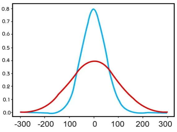
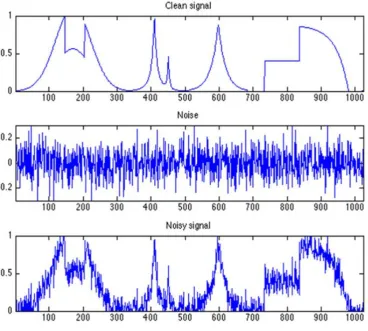
Figure 5. Variability, noise and stimulus information. Here using an example of radio signals we show the effects of factors such as the weather and neural noise might have on ‘clean’ stimulus information. Radio signals are an apt simile to visual signals as they are much the same as light signals. The only difference in the
wavelength of the waves which are subject to many of the same sources of noise and variability. In the upper panel is a ‘clean’ radio signal. The variability in the frequency of this signal carries information about the content of the information transmitted by the sender. On its own interpretation of the clean signal is
straightforward as the signal carries only variability about the signal of interest. In the middle panel we have only noise. Noise is unrelated to the radio signal carrying stimulus information. In radio waves, like light waves, noise can arise from atmospheric conditions or noise from other task irrelevant signals such as from other radio waves transmitting in a similar channel. It can also arise from components in the radio such as the flow of charges in the radio device (much like neural noise). The lower panel illustrates the sum total of signal and noise which must be interpreted by the receiving device. As we can see the addition of noise makes the radio signals of interest much more variable, which makes the true signal more uncertain and harder to interpret (figure adapted from signal and noise
1.7. Variability in signals and measurements produces little effect on perception and behaviour: application of prior knowledge.
The internal and external sources of variability we have presented are certainly not trivial. It is apparent that the information that reaches the cortex about stimuli in the world is very often or most likely always variable making interpretation of important stimulus information constantly uncertain to some degree. Given the nature of the factors which produce uncertainty in visual information we might logically expect certain effects of different sources of variability to be present in perception. Because we constantly need to blink we might conclude that they would seriously interrupt our flow of visual consciousness. In addition, we might also expect our perception of objects in the world to be unstable nearly all of the time due to constant retinal instability or perception in bad weather or poor light to be worse than it actually is. Furthermore, we might think that neural noise would lead to confusion in the interpretation of incoming signals as it adds random fluctuations to the incoming information. However, in reality both internal and external variability appear to exert little effect on perception and behaviour in normal circumstances. We barely notice blinks despite occurring almost constantly, perception is remarkably stable at all times and our perception in bad weather and poor light although somewhat decreased in acuity is still normally reliable enough to perceive relevant stimuli and respond accordingly. Therefore, the contrast between the variable nature of visual information received at the cortex and our subjective visual and behavioural experience raises an important and currently unanswered question. Specifically, what computational processing strategies is the visual cortex applying to its inputs to extract relevant stimulus information from the mass of uncertain visual information emitting from world and turn this information into the high grade perceptions we are familiar with.
Exactly how the brain reconciles uncertainty is not fully understood. However, one strategy the visual system does appear to employ is to apply prior knowledge to interpreting current visual inputs
(Friston, 2010; Kok, & De Lange, 2016). Importantly, the application of previous experience to current visual inputs rests on certain rules and characteristics present in the physical world and the way stimuli behave (Chun, 2003; Turk-Browne, 2012). Events and the behaviour of stimuli in the natural world rarely evolve completely randomly. Usually, the way events unfold and the way stimuli behave exhibit temporal regularities and relationships which can potentially be learnt and applied when interpreting variable visual information (de Lange, Heilbron, & Kok, 2018). One aspect of temporal structures and regularities that is very important to emphasise, is that such structures and regularities exist at varying levels of complexity (Barlow, 2001; de Lange, Heilbron, & Kok, 2018; Turk-Browne et al, 2009) which effects how they might be utilised by the brain.
1.8. Types of temporal regularity.
are often repeats of one another (Fischer & Whitney, 2014; Liberman, Fischer, & Whitney, 2014; Liberman, Zhang, & Whitney, 2016). While we may not really think much about temporal stability as objects that are stable tend not to be behaviourally pressing, stability is nonetheless extremely
prevalent. Examples of environmental stability are practically everywhere. If you look around your office or place of work right now, it is highly likely that very little is changing. Walls and windows remain in the same place, your desk does not suddenly appear in another part of the room and a book left on a shelf remains in the same location unless moved. Temporal stability can also occur in the behaviour of many stimuli in which the actions are simple repeats of themselves. The way people walk follows a similar pattern and the way a key goes into a lock and almost always turns clockwise provides past information that can be used to help minimize uncertainty. A commonly stable environment and repeated common behaviours means that in some instances a good estimate of a stimulus value of interest within a stream of noisy visual information is that next value will be the same or similar to the current values, at least over a short to medium time span, or that an action or event we have just observed will be repeated again.
In addition to an unchanging world or the simple repeats of behaviours a different type of temporal regularity are the conditional probabilities that exist between stimuli and events in the world (de Lange et al., 2018; Friston, 2010). For example, one simple type of conditional relationship are cues that signal a certain outcome. If you cook food in a microwave and the buzzer sounds we can make a judgment that as we have heard the buzzer our food is cooked. Importantly, more complex conditional relationships also exist within sequences of events that evolve over time. If you walk through a busy train station, you need to negotiate your way through lots of people many going in different directions heading to different exits to get onto your required train. Here, there are potentially many different paths people could take. One way to predict the position of other people and where they might be next might be by combining sequential information about how people will transition from the current to a future position based on the previous n-1, n-2, n-3, n-4… time points combined with knowledge of the exits and entrances of the station. By using conditional relationships provided by cues and sequences of events in our surroundings it is possible to decrease the level of uncertainty of sensory information which if judged on an independent basis might be subject to misinterpretation or errors (de Lange et al. 2018).
provide some excellent examples for the general idea of temporal integration in visual perception and also highlight some limitations in the understanding of the exact type of strategies by which the visual system exploits such regularities
1.9 Broad evidence that the visual system integrates temporal structure when interpreting variable retinal measurements.
An area of serial effects research that provides a good illustration of temporal integration comes from visual masking. Visual masking refers to the phenomena that the current perception of a target stimulus is reduced by the presence of another stimuli called a mask (Breitmeyer & Ogmen, 2000). With respect to time three types of masking are usually tested; forward, backward, and simultaneous. In backward visual masking a target stimuli is presented for a short period of time and followed quickly by the “mask” (Kahneman, 1968). In suitable temporal conditions, the trailing mask can greatly reduce the perception of the target stimulus, even though the two visual events are separated in time (Breitmeyer & Ogmen, 2000; Kafaligonul, Breitmeyer, & Öğmen, 2015).The fact that the mask exerts an effect on the perception of the target even though the two events are distinct in time has been taken in support of the idea that the visual system retains a representation of the stimuli which it integrates in some way with the current retinal image (Breitmeyer & Ogmen, 2000). Because the two images are combined the perception of the current image is less accurate as it also contains
information from the previous measurement (Breitmeyer & Ganz, 1976; Breitmeyer & Ogmen, 2000; Swift, 2013).
integrates information from images observed in separate time windows to help create a coherent image of two uncertain half or interrupted images.
An especially well studied phenomena studied under the umbrella of serial effects that illustrates the way past information can improve the effectiveness of behaviour is repetition priming. Repetition priming is a phenomena in which the behavioural response to a stimulus, usually measured in reaction times or accuracy, is improved by the repeated presentation of a stimulus (Kristjánsson, 2006;
Yoshimoto et al., 2013). A number of priming of pop out tasks have provided strong and illustrative evidence for the contextualizing and performance enhancing input of previously observed stimuli. Commonly, in priming of pop out studies participants are asked to search for a stimulus of odd dimensions such as colour or shape relative to distractor stimuli of a similar but distinct nature that have another distinguishing feature such as a notch missing or an orientation marker (Becker, 2008; Goolsby & Suzuki, 2001; Maljkovic & Nakayama, 1994; Magnussen & Greenlee, 1999; Olivers & Meeter, 2008). Participants are then asked to state the nature of the distinguishing feature, i.e. is the notch to the right or the left or what orientation is the marker on the stimulus. Results normally report that if the target stimuli shares colour or shape with the previous target stimulus, even if the
distinguishing feature that they are asked to report on is different, then reaction times are decreased or accuracy improved (Becker, 2008; Goolsby & Suzuki, 2001; Maljkovic & Nakayama, 1994)
Crucially, because the priming observed is separate to the task demands then it might be interpreted as participants interpreting potentially uncertain information based on an integration of the salient features in stimuli.
opposed to simple repeats. Also, such empirical findings level studies do not touch on the underlying computations of integration or what the aim of integrating actually is. Is the aim of integration simply to increase signal to noise ratio or to actively reduce the amount of error in perception and responses which while appearing to be similar goals potentially arise from different computational strategies. Overall, on the basis of such research it could be valid to say that the visual system does integrate information over time but that it is also reasonable to say that such empirical research gives no theoretical explanation of the factors which mediate integration and the underlying computations that underpin integration or what the actual aim of integration might be.However, while much serial effects research does function at the empirical level there do exist ideas which do provide theoretical explanations of the how and why the brain integrates information over time.
1.10 Two predictive integration strategies: assume stability and predict based on the average of values observed over time or learn the conditional relationships between stimuli and predict. Theoretical ideas about how and why the visual system integrates information about the statistical regularities of the environment have long concerned the thoughts of some of the most important figures in the history of cognitive science. These figures include including Helmholtz, Mach, Pearson, Craik, Attneave, Barlow and Gregory giving a clear indication of the level of such research. Due in no small part to the ideas of such crucial figures, an important idea has emerged within cognitive science. This idea, is that in order to help resolve uncertainty the brain makes forecasts or predictions about the content of its variable inputs based on past experience. Here though, it is important to raise an
important point central to the current thesis. That is that the term prediction can be used in a number of ways and there is also more than one way to make a prediction. Over time a number of strategies about how the brain might predict the nature of its uncertain inputs have emerged and here we focus on two of them. Namely perceptual averaging (Corbett, Venuti, & Melcher, 2016) and perceptual inference derived mainly from the early works of Helmholtz (1867).
1.11 Perceptual averaging and perceptual inference.
Perceptual averaging is a simple way to make a prediction about variable measurements familiar to anyone who has worked with interpreting noisy signals that relies on a simple underlying assumption. This assumption is that there is some level of temporal stability in the stimulus under measurement but that measurements are also variable to some extent. Under this expectation a good way to predict a stimulus value is to base predictions on an average of values observed over time. Importantly, this type of prediction is while still a prediction more of a retrodictive type of prediction and relies on past information entirely. Perceptual inference on the other hand also involves a type of averaging to resolve uncertainty but in this case averaging also makes use of some of the more complex type of conditional sequential relationships present in the environment and is perhaps a more ‘true’ or
present in more complex sequential information arising from the way stimuli behave or events occur in the world. Also, the time frames from which such learnt sequential and contextual knowledge can be applied to interpreting current sensory inputs can potentially be garnered from not only the previous seconds but potentially from much longer time frames. Crucially the ability to incorporate complex sequential relationships allows the construction of complex mental models that simulate future states of the environment based on how we expect the world to behave in the future in a more prospective manner (Friston, 2010). Examples which can help to distinguish the difference between perceptual averaging and perceptual inference can be observed in many day to day situations.
Fixed rate perceptual averaging is a term that can be applied to explain the finding that people’s perceptions of current stimuli appears to revert towards the mean values of previously observed stimuli (Albrecht & Scholl, 2010; Albrecht, Scholl, & Chun, 2012; Jones & Dekker, 2018). Mean reversion is a century old finding first recorded in an experiment which showed that participants frequently choose a probe card that was too large when the cue card was small compared to the other cards presented in the experiment and selected a probe card that was too small when the cue card was larger (Hollingworth, 1910). Current findings indicting similar averaging behaviours come from both the spatial domain, in which the perception of a stimulus ensemble appears to represent the mean of shapes and sizes of objects in the current field of view (Campbell & Robson, 1968; Corbett,
Wurnitsch, Schwartz, & Whitney, 2012a; Parkes, Lund, Angelucci, Solomon, & Morgan, 2001) and in the temporal domain in perception appears to represent a reversion to the mean of stimulus values observed over time, a phenomena often termed serial dependence (Alais, Leung, & Van Der Burg, 2017 ; Cicchini et al., 2014.; Corbett, Fischer, & Whitney, 2011; Kiyonaga et al., 2017; Liberman, Fischer, & Whitney, 2014; Liberman, Zhang, & Whitney, 2016; Moors, Stein, Wagemans, & Ee, 2015).
Serial dependence is defined as bias in participant’ judgments of a current stimulus value towards the mean of previous stimulus values (Fischer & Whitney, 2014). In serial dependence literature, mean reversion is interpreted under an internal assumption of a stable environment in which measurements at the retina are always uncertain to some extent (Fischer & Whitney, 2014). The general idea behind the function of serial dependence is that by representing perception as the fixed mean of values observed over time, variability in visual information from factors such as blinks and saccades are smoothed over allowing more accurate representations of the true values of stimuli of interest than those provided by a single uncertain measurement (Liberman et al., 2016; St. John-Saaltink et al., 2016). However, like any method of averaging or indeed statistical interpretation the implied fixed weighted method has its disadvantages and there are additional problems in regard to the way the fixed average account of temporal integration is somewhat less than clearly described in the literature.
variable then basing perceptions on a fixed average of past measurements means perceptions will not be indicative of the current state of signal as the perception is anchored on past measurements making them lagged in time to large changes in stimuli value. Also, the implied fixed average method of perceptual averaging suffers from a lack of an explicitly stated mathematical or computational model by which to guide experimental design and compare against other computational account of temporal integration. It appears that the general explanation of serial dependence is based on fixed weighted average models commonly used in signal processing but this is never actually stated. Without an explicitly stated computational account it is difficult to design experiments which test the fixed account of integration or compare against other accounts of temporal integration such as predictive coding which do have a more formalised if varied computational structure.
1.12. Predictive coding account of temporal integration: basic ideas
Predictive coding is a major theoretical movement within cognitive science and potentially represents a considerable paradigm shift in the way we think about vision (see Clark, 2013) for an overview of predictive coding theory). The general idea of some current and highly influential predictive coding models is that is that the visual system contains a series of hierarchical internal model(s) (Friston, 2010; Spratling, 2015). Each layer of the hierarchy contains an increasingly complex (from lower to higher) representation of the statistical regularities of the spatial structure and temporal regularities of the world. Based on the general parameters of the internal models the visual system constantly extrapolates or predicts the origin and cause of its expected neural and sensory activity such that superior hierarchal levels make predictions about activity at inferior levels via top down signals. Differences between predictions and measurements produce error or ‘prediction error’ signals which are sent back up the hierarchy to update the internal model and the subsequent predictions according to the nature of the prediction error.
In the literature, terms such as measurement and prediction can be used somewhat loosely so we define some important terminology. Here, we define prediction as an estimation of what the next sensory measurement will be. A measurement can be from the world as made by retinal ganglion cells as we have defined previously but in predictive coding also within early cortical regions (Friston, 2010). The next estimation can be next in time or in space. However, one very important aspect of predictive coding to be aware of is that predictive coding is essentially a computational motif. The term predictive coding simply means a neural process involving prediction and prediction error (Aitchison & Lengyel, 2017) and there are certain aspects of predictive coding that could be
perceptions while at the same providing a ‘default model’ of predictive coding to highlight some of the differences between predictive coding models comes from Rao & Ballard (1999).
1.13. Rao and Ballard (1999) predictive coding in sensory cortex model.
Rao and Ballard’s (1999) computational framework provides a specific illustration of the nature of predictive coding’s hierarchical models and how the prediction, measurement, prediction error and update cycle function in the spatial prediction of image intensities. In Rao & Ballard’s (1999) hierarchal model, each level contains a representation of the spatial structures of an image intensities within an image. Each level in the hierarchy has an increase in receptive field size dealing with increasingly larger and complex areas of the image. In a three-level predictive coding model, level 0 will consist of a group of modules which deal directly with the measurement. Level 2 receives input from all the modules of Level 1 and at the same time feeds level 1 with prediction signals based on the probability of surrounding pixel intensities, while level 3 receives input from level two and at the same time predicts activity at level two. This hierarchical system functions throughout Rao & Ballards (1999) framework, with the highest level having the potential to receive input from all areas of the visual field and predict the whole image for the lower levels. Importantly, this cycle of prediction, measurement, comparison and prediction error happens constantly and with each iteration prediction error is reduced and predictions refined as more and more predictions and measurements are
Figure 6. Schematic illustration of Rao & Ballard’s (1999) predictive coding model.
Another key concept of predictive coding that is covered in Rao & Ballard (1999) is how to weight prediction errors, a term they call optimization function. For prediction errors to be a useful basis by which to inform and update perceptions they must recognize the variable nature of the natural world. For instance, greater confidence should be assigned to prediction errors in broad daylight than errors in prediction at nightfall (Hohwy, 2012). In Rao & Ballard (1999), prediction errors are weighted based on the inverse variance of the squared error between the current prediction and the mean of past measurements, such that a low sum of squares indicates a reliable prediction error while a larger sum of squares indicates less reliable prediction errors. With a higher level of reliability, internal models update and alter subsequent predictions by a larger amount relative to the size of the prediction error and with lower reliability the internal model updates and alters subsequent predictions by a smaller amount relative to the size of the prediction error. Importantly, the way prediction errors are weighted, varies between predictive coding models but normally involves the weighting of variances in
prediction errors or measurements in some way and is adaptive to the setting in which predictions are made.
1.14. Missing pieces of the predictive coding puzzle: temporal predictive coding model and explicit perceptual averaging model.
some areas of areas of predictive coding and perhaps contributed to some areas of visual processing including our area of interest, predictive coding in time, missing a specific account of predictive coding altogether.
In predictive coding literature, in addition to Rao & Ballard (1999), there exist models for predictive coding in the retina (Hoyosa & Meister, 2005), Spratling’s PC/BC-DIM model (Spratling, 2015) again for spatial predictive coding and more general predictive coding models such as Fristons’s free energy model (Friston, 2015) and linear predictive coding (Makhoul, 1975; O’Shaughnessy, 1988). Importantly, none of these models apply to the temporal domain directly. Also there are confusing accounts of the nature of the internal modelsprobabilistic representation. The dominant predictive account is one of a hierarchical system based on conditional probabilities under Bayes optimal principles such that interpretation of activity at lower levels is conditioned by those above them (Clark, 2013; Friston, 2011; Friston et al., 2002). Rao & Ballards (1999) model also involves a hierarchical system seemingly implying the use of conditional probabilities but is primarily a linear model with no real need for complex conditional relationships and indeed never actually mentions conditional probabilities. Furthermore, exactly how prediction errors are weighted is often ignored in studies examining predictive coding in time. Again Rao & Ballard (1999), provide one way of weighting prediction errors, based on the inverse variance of errors but their method is based only on computational simulations of a model for spatial predictive coding. Overall, conflicting accounts of how predictive coding might be realised combined with a lack of a specific model for predictive coding in time highlight missing pieces of the predictive coding ‘puzzle’.
The lack of a specific model for predictive coding is an important piece of the predictive coding puzzle that is currently missing. While we have discussed other models of predictive coding in the spatial domain and more general models this is not intended so much as a critique but simply to highlight the idea that there are potentially a number of ways predictive coding might be implemented depending on the sensory domain in question. There is no doubt that models such as Rao & Ballard (1999) and those from Spratling (2015) and Friston (2010) are excellent accounts of predictive coding but by its very definition the term ‘prediction’ applies to time. Indeed, it is the easiest type of
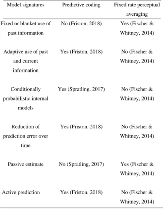
1.15. Lack of specific computational temporal models make the behavioural signatures of fixed weighted perceptual averaging and predictive coding difficult to identify in current literature Conceptually, predictive coding and fixed rate averaging appear markedly different. They each have contrasting aims, integrate different types of information and have different levels of complexity. However, due to a lack of clear and testable computational models by which to guide experimental designs it is open to question whether results interpreted under a fixed perceptual averaging in serial dependence literature have been correctly interpreted and also perhaps even more importantly whether predictive coding in time has been adequately distinguished (see table 1 below) . In order to illustrate the problems in experimental design caused by the lack of an explicit computational accounts of fixed perceptual averaging and the lack of an accepted model for predictive coding in time now we provide examples of current literature that highlights the nature of this problem.
Table 1. Predictive coding versus fixed rate perceptual averaging Model signatures Predictive coding Fixed rate perceptual
averaging Fixed or blanket use of
past information
No (Friston, 2018) Yes (Fischer & Whitney, 2014)
Adaptive use of past and current information
Yes (Friston, 2018) No (Fischer & Whitney, 2014)
Conditionally probabilistic internal
models
Yes (Spratling, 2017) No (Fischer & Whitney, 2014)
Reduction of prediction error over
time
Yes (Friston, 2018) No (Fischer & Whitney, 2014)
Passive estimate No (Spratling, 2017) Yes (Fischer & Whitney, 2014)
1.16. Fixed weighting of past and current measurements or not? Ambiguity in serial dependence research.
Perceptual averaging in the temporal domain is often termed serial dependence. Presently, serial dependence is an increasingly popular area of vision science which examines the nature of the observed bias or dependence of current perceptions on past stimulus values. Within an influential section of serial dependence research, it has been implied that serial dependence functions as a form of a fixed weighted average model in which the weights applied to measurements of past and current stimulus values included in perceptual estimates always remain at a fixed level (Fischer & Whitney, 2014; Liberman et al., 2014, 2016). If this idea is correct, a number of key identifying factors should exist in the current perceptual estimate of a stimulus value. One is that there should always be some influence of previous stimulus values in any current perception of a stimulus value. Another
potentially identifiable hallmark, is that because the fixed account of serial dependence operates under a very simple assumption of a constantly stable but uncertain world the model does not include any concept of how the reliability in our perceptions of a stimulus or how the behaviour of a stimulus itself might affect integration and does not adapt perceptions to such situations. This means that the behaviour of a stimulus and how reliable the perception of a stimulus is does not affect serial
dependence in any way. However, based on current serial dependence literature it appears that results from serial dependence studies may also be interpreted under at least the general principles of
predictive coding which posits a more adaptive integration strategy.
Fischer & Whitney (2014), examined serial dependence in the perception of orientation. Their task involved presenting a series of orientated Gabor stimuli for 500 ms and then asking participants to estimate the orientation of the Gabors they has just seen by moving an adjustment bar (see figure 7 for a more detailed illustration) Interestingly, Fischer & Whitney (2014) claimed findings consistent with a fixed account of temporal integration and observed a bias in the judgment of both fully random and more stable counterbalanced Gabor stimulus orientations. One caveat with this interpretation is that the level of dependence while always present to some extent does appear to have been influenced by the variability of orientations and the level of variability in the measurement of the stimulus. When Gabor orientations had radically different orientations from previous orientations judgments serial dependence decreased and when orientations were more similar serial dependence increased indicating a role for stimulus variability. Another interesting aspect of Fischer & Whitney (2014) experiment is that while Gabor stimuli had a relatively high contrast (25% Michelson), the stimulus also had a relatively low spatial frequency (0.33 cycles per degree). The effect of low spatial
frequency was to make Gabor orientations blurred. Blur has been shown to make judgments of stimuli more variable, quite feasibly due to an increase in measurement variability at the cortex (Kayargadde et al, , 1996 ). Furthermore, the use of a noise mask in between stimuli and judgment trials and
contributed to increased measurement variability. These factors are important because if the role of measurement variability is a factor in temporal integration as in predictive coding (Friston, 2010; Gordon et al., 2017), it may be possible that the weighting attached to any prediction errors caused by the change in the Gabors orientation did not carry enough weight to update the new prediction to its full amount. If the prediction was not updated to the full amount of the prediction error then it may appear that the perception lies somewhere between the past and current stimulus measurement and appears serially dependent. However, in order to test the role of stimulus variability and measurement variability a more rigorous experimental manipulation that takes into account these factors is required.
Figure 7. Fischer & Whitney’s (2014) experimental design and task. Participants viewed a Gabor stimulus presented wither to the left or right of fixation interrupted by a noise mask and reported the perceived orientation of the Gabor by adjusting the orientation of a response bar.
Results showed that when positions of the target stimuli were more similar to previous targets serial dependence increased and decreased when further apart. Also, when the inter trial mask was removed no serial dependence was observed. Manassi et al (2018) acknowledges this result and explains it under the idea that the time reduction of the inter trial interval, reduced by the removal of the mask, was the causal factor but offers no theoretical explanation why this may be the case. A potential predictive coding explanation why serial dependence dropped out, is that when the mask was removed the level of measurement uncertainty in the weighting of any prediction error between the previous and current stimulus positions was reduced, meaning any error in the prediction of the current positions is weighted as being more reliable. With a more certain prediction error, it is possible that the current perception was corrected to the full extent of the prediction error produced by the change in stimulus positions. With a total correction to the new measurement no influence of previous stimulus values would be detected in the response and thus no serial dependence. Again though, such an interpretation is speculative and because the paper does not actually state that averaging is always fixed and does not provide any explicit model of the type of averaging implied it is hard to critique the findings in terms of the fixed weighted average theory.
A further interesting serial dependence study that could be subject to dual interpretations is Liberman, Zhang & Whitney (2016). This study examined the role that serial dependence has in interpreting partially occluded stimuli under the premise that integrating measurements over time helps to maintain a coherent perception when measurements are incomplete (Fischer & Whitney, 2014). Participants were tasked with judging the orientation of a partially occluded Gabor stimulus that was presented as either as continually moving or as a discontinuous series of orientations. Results again showed that serial dependence increased when orientations were more similar and decreased when further apart. Interestingly, and again providing contradictory evidence with a fixed weighted average account of serial dependence, in the discontinuous condition no serial dependence was observed. As no serial dependence was observed under more variable stimuli conditions this result could again be interpreted under a predictive coding or certainly adaptive accounts of integration in which the level of variability in measurements and stimulus behaviours play a role in updating predictions.
1.17. Predictive coding in time, or alternative explanations?
In a similar fashion to the way the fixed account of serial dependence research has been subject to a lack of clear theoretical guidance when designing adequate experimental designs, predictive coding in the temporal domain can also be considered to be subject to a similar problem. Within temporal predictive coding literature to date no concrete computational model has been tested and compared to the behaviour of human participants. Due to a lack of a clear and testable theory by which to base experiments upon it is open to question whether key aspects of predictive coding such the adaptive weighting of prediction errors have been tested fully in purely visual term. Furthermore, and perhaps most importantly, there are also questions about the type of probabilistic representations and
complexity of information used to make predictions. To illustrate the limitations related to a lack of a clear theoretical model for predictive coding in time we provide evidence from a number of predictive coding studies that have claimed to observe predictive coding in time and debate the interpretation of such findings.
A neural phenomena that has been utilised to support the idea that predictive coding applies to the temporal domain is repetition suppression. Repetition suppression is defined as the diminished neural activation that results from the repeated presentation of a stimulus over time (Henson, 2003; Wiggs & Martin, 1998). Explanations for repetition suppression are keenly debated. The original explanation for repetition suppression was that reduced activity neural patterns could be explained by simple fatigue effects (Grill-Spector, Henson, & Martin, 2003) . By this account, the attenuation of a neural response is hypothesized to be due to an overall reduction in a neuron's firing rate as the neurons expend their energy or neurotransmitters. An alternative explanation of repetition suppression advanced by supporters of predictive coding, is that overall neural activity at lower levels of predictive coding’s hierarchy is reduced by top down driven prediction signals when they are congruent with expected activity (Auksztulewicz & Friston, 2016; Grotheer, 2016a). Over time a number of studies have tested the predictive coding account of repetition suppression by manipulating the predictability of stimuli.
face images were trial unique which ensured that the probability of a repetition and not the repetition of a particular face was manipulated. As an incidental task was while observing trials, participants were asked to respond to occasional inverted faces the aim of which appears to have been to keep participants ‘on trial’.
Summerfield Trittschuh, Monti, Mesulam, & Egner (2008) reported some interesting findings. Firstly, in high probability blocks BOLD signal was decreased with repeated trials in these blocks producing a decrease in BOLD signal of around 22% compared to alternation trials. In low probability blocks, repetition trials elicited only a reduction of 9% in BOLD signal compared to alternation trials. Statistical analysis showed a main effect of trial type on BOLD signal and more importantly a significant block type and stimulus interaction effect on BOLD signal meaning that the both the overall probability of seeing a repetition and actually seeing a repetition had an effect on BOLD signal. In terms of behavioural responses, reaction times to target inverted faces reported no significant difference between blocks. Summerfield et al (2008) concluded that the expectation of both stimulus repetition and block probability were both predictors of repetition suppression, with the context provided by block probability level superseding simple stimulus repetition. However, while results reported that the probability of a repetition and a repetition itself did reduce BOLD signal there are a number of questions related to the design and interpretation of the study with some aspects of Summerfield et al (2008) predictive coding interpretation of results open to debate.
One question arises from the type of ‘predictions’ in the behavioural aspect of the study. This is because participants were presented with a reliable cue. While it is of course still possible to make a prediction about the current input based on a cue but the use of cues can be thought of as providing a more simple associative relationship as opposed to a more ‘forward’ type of prediction about what will happen next based on sequential conditional probabilities. Perhaps some behavioural measure of what participants ‘expected’ was going to constitute the next face image should have been added to the study by inserting conditional relationships between stimuli into the sequences of trials and omitting trials and then asking for a prediction about the next trial might have been a better design. Another critique is that the study does not include any notion of the difference between the
measurement of the stimuli in the world and the actual signals stimuli produce. In a number of influential predictive coding models, when the measurement of the stimulus is less certain the weight attached to prediction errors is downgraded (Friston, 2018; Spratling, 2015). Presenting clearly visible stimuli cannot, therefore, test this notion. In addition, due to the rather simple probabilities assigned to blocks and trials, it is open to question whether the neural activity changes observed between high and were due to the probabilities of observing repetition or alternation trails. A possible alternative
changes producing more neural activity. A final criticism that also provides a basis for a fixed weighted average integration interpretation of Summerfield et al (2008) results, is that even when stimulus repetition was rare repetition suppression was never totally absent. In a fixed average account some trace of past stimulus measurements always persists as the current estimate always contains at least some past stimulus history. The persistence of repetition suppression could reflect the persistence of past values as would occur with a fixed weighted account but in predictive coding this does not have to be the case. An attractive aspect of predictive coding is that given the correct conditions all past stimulus history can be discarded and the response will equate to the current stimulus which in theory should extinguish repetition suppression entirely. However, as the design of the experiment did not manipulate the reliability of sensory measurements (how well participants could see the stimulus) the experimental design was not adequate to test this aspect of the predictive coding.
An illustrative account from predictive coding literature that further illustrates the ambiguity in ascertaining which integration strategy has actually been performed comes from Summerfield & Koechlin (2008). In this study, the researchers aimed to manipulate predictions and predictions errors in upcoming stimuli orientations by providing them with specific perceptual templates that drew upon two classical psychophysical tasks. Task 1 was a two alternative forced choice task called the A/B task, because participants were shown two orientation lines of different colours (A, red & B, blue) on a grey circle separated by 60° on the same stimulus and then asked to report if the grating of a subsequently presented Gabor stimulus was the same as A or B . The second task was a yes/no type paradigm, in which they were only shown the A orientation and then asked to state whether the orientation of the next subsequently presented Gabor stimuli matched the A orientation or not (~A). Of total trials 50% of target Gabors in the A/B task were A and 50% B. Also in the A/~A task, 50% of the targets were A and 50% were ~A. The type of the target changed randomly from trial to trial in both tasks and trials were presented inter leaved blocks of A/B and A/ ~A.