Using Topic Models in Content-Based News Recommender
Systems
Tapio Luostarinen
1, Oskar Kohonen
2(1) Comtra Oy, Savonlinna, Finland (2) Aalto University School of Science
Department of Information and Computer Science, Finland
[email protected],[email protected]
A
BSTRACTWe study content-based recommendation of Finnish news in a system with a very small group of users. We compare three standard methods, Naïve Bayes (NB), K-Nearest Neighbor (kNN) Regression and Regulairized Linear Regression in a novel online simulation setting and in a cold-start simulation. We also apply Latent Dirichlet Allocation (LDA) on the large corpus of news and compare the learned features to those found by Singular Value Decomposition (SVD). Our results indicate that Naïve Bayes is the worst of the three models. K-Nearest Neighbor performs consistently well across input features. Regularized Linear Regression performs generally worse than kNN, but reaches similar performance as kNN with some features. Regularized Linear Regression gains statistically significant improvements over the word-features with LDA both on the full data set and in the cold-start simulation. In the cold-start simulation we find that LDA gives statistically significant improvements for all the methods.
1 Introduction
With online news it is possible to read a large amount of different news sources on a large array of topics, but since there are more articles available, finding interesting ones becomes more difficult, as reading even just every headline becomes cumbersome. Consequently automatic filtering with recommender systems, becomes attractive. We consider the specific problem of how to build a news recommender system to find interesting news within a specific language group, Finnish. We use content-based recommender systems, which is the less studied of the two main paradigms of recommender systems (Adomavicius and Tuzhilin, 2005). The main benefit of this content-based recommendation is that it allows others than large user communities and their parent companies to build recommender systems for any material they want to, also any niche content, be it by language, topic or anything else. By contrast, collaborative filtering requires a large user community, since it bases its recommendation on how similar users have rated the items. Another problem for news recommendation and collaborative filtering is that, even if there is a sufficient number of similar users, the items need to have been rated by at least some of these users, and in the case of news recommendation, it is the new items which are most interesting, and these are the ones least likely to have been rated. Because of this, news recommendation systems usually include content-based recommendation, where items are recommended to users based on a profile of what kind of content the user has liked in the past (Lang, 1995; Billsus and Pazzani, 2000).
Because our collected data is from a small community of users, we concentrate purely on content-based recommendation. We consider the case where users provide explicit ratings of how well they liked the content, rather than using the implicit feedback based on their reading behavior. We compare three standard methods, Naïve Bayes (NB), K-Nearest Neighbor Regression (kNN) and Regularized Linear Regression (Lin), which have all been suggested earlier in the literature, but no comparison seems to be available.
Since we have comparatively few ratings, but a large corpus of news, a natural extension is to apply unsupervised learning to the unrated news and discover features that reflect the statistical structure of news items. These discovered features can then be used to improve performance of the supervised recommender system. While this is a common approach in machine learning, it has not been applied to content-based recommender systems. We apply Latent Dirichlet Allocation (LDA) (Blei et al., 2003) and compare the learned features to those found by Latent Semantic Indexing (Deerwester, 1988).
To motivate a user to keep using a recommender system, it needs to provide recommendations already with very few rated items. This is known as the cold-start problem (see e.g. (Schein et al., 2002; Rashid et al., 2008)), and we study how the amount of ratings affects recommendation performance.
2 Related Work
Content-based news recommendation has been addressed in the literature by several authors. Lang (1995) describes a method combining nearest neighbors and linear regression, using a combination of TF-IDF features and features selected with Minimum Description Length (MDL). Billsus and Pazzani (2000) used a combination of Nearest Neighbor Classification and Naïve Bayes classification for explicit feedback in an interesting/not interesting classification. In contrast to this work, we use the methods as straightforward predictors, rather than in combinations, and we use a rating on the scale 1-5. Naïve Bayes has also been applied to
content-based book recommendation (Mooney and Roy, 2000).
Topic models have not been used directly in content-based recommendation with explicit feedback, but with implicit feedback, a method similar to probabilistic Latent Semantic Indexing (Hofmann, 1999) has been applied by (Cleger-Tamayo et al., 2012). The topic model used is adapted to user behavior. We don’t consider topic model adaptation, but rather use Latent Dirichlet Allocation (Blei et al., 2003) as an unsupervised feature extraction procedure. We argue, that while adaptation is likely to be useful for users with many rated items, lower dimensional features from topic models are most interesting in the cold-start situation when it is difficult for the methods to fit to a high-dimensional content vector.
Rashid et al. (2008) derive information theoretic strategies for how the first recommendations for a new users should be made. In our work, we will merely measure the cold-start performance of the methods, to assess how different methods work with very few rated items.
Recommender systems are increasingly seen as ranking problems, since we are trying to suggest the most relevant items to the user (see e.g. (Takács and Tikk, 2012)). However, the methods that we consider, reduce the recommendation problem to predicting the user ratings, since this allows simpler methods. We do agree that ranking performance is more important than prediction performance, and therefore we evaluate also ranking accuracy.
3 Methods
We implement the recommender systems separately for each user. For each user we have a training set of documentsdi ∈ D that the user has assigned ratingsr(di)∈ {1, 2, 3, 4, 5}. The documents are represented by feature vectors, where the feature set is denotedV. We implement the recommender methods in two ways. Firstly, as a five class classification task, where the classes correspond to the ratings 1-5 or, secondly, as a regression task, where the rating is seen as a continuous value to be predicted. The former is used in combination with Naïve Bayes, and the latter with K-Nearest Neighbors and Regularized Linear Regression. The latter approach suffers from the problem that the method may assign scores outside the scale 1-5. This is however irrelevant when ranking documents.
3.1 Naïve Bayes classification
We implement the Naïve Bayes classifier following (McCallum and Nigam, 1998), where documents are modeled as sequences of samples drawn from a multinomial distribution of words, with as many independent draws as the number of words in the document, each class having its own multinomial distribution. Here, as the class represents the rating, we denote it
rj, where j∈C={1, 2, 3, 4, 5}. The word probability parameters can then be calculated from the labeled data:
P(di,k|rj;θˆ) =
P|D|
i=1di,kP(rj|di)
P|V |
s=1
P|D|
i=1di,sP(rj|di)
(1)
Bayes’ rule.
ˆrN B(dnew) =arg maxr0∈CP(rj|d) =arg maxrj∈C
P(rj)P(d|rj)
P(d) =arg maxrj∈CP(rj)P(d|rj) (2)
3.2 Nearest Neighbor Regression
Nearest neighbormethods are very simple to implement and they can be used for both classifica-tion and regression. They simply store in memory all the training samples and the outcome for a new sample is based solely on thenearest neighbororknearest neighbors in the training set. The nearest neighbor is selected as the most similar sample:
d0=arg max
di∈D
sim(di,dnew) (3)
wheresim(di,dj)is the similarity measure being used. The performance of the nearest neighbor methods depends significantly on the similarity measure. We used cosine similarityas the measure and it is defined as (Salton, 1989):
sim(di,dj) =cos(α) =
P|V |
k=1(di,kdj,k)
qP|V |
k=1di,k2
qP|V |
k=1d2j,k
(4)
Letdj,j=1, ...,kbe the set ofknearest neighbors for the itemdnew. We calculate the value for a new item as a weighted average of theknearest neighbors (Billsus and Pazzani, 2000):
ˆ
rkN N(dnew) =
Pk
j=1r(dj)×sim(dnew,dj)
Pk
j=1sim(dnew,dj)
(5)
3.3 Regularized Linear Regression
The basic idea of linear models is to find in some sense optimal coefficientsβkfor each variable
di,kin the linear equations:
ˆ
rLin(di) =β0+
|V |
X
k=1
βkdi,k (6)
The recommender system we are building should be able to present some recommendations even with just a few rated items, so we used a regularized least squares formulation, which can be applied with only a few samples. We usedelastic net, a combination oflassoandridge
regressions. This model still minimizes the squared errors, but the coefficients are regularized by both L1-norm and L2-norm. The regularization part of the expression can be stated with
a scale parameterλand a linear weight parameterα∈[0, 1]to select between L1-norm and
L2-norm (Friedman et al., 2010):
ˆ
βelastic=arg min
|D|
X
i=1
r(di)−(β0+X|V |
k=1
βkdi,k)
2
+λ
|D|
X
i=1
1
2(1−α)βk2+α|βk|
(7)
Zou et al. (Zou and Hastie, 2005) have also shown that elastic net, in case of highly correlated variables, tends to select all of them at once or leave them all out at once. Studies have shown that this kind of grouping effect clearly improves the prediction accuracy of linear models compared to lasso when there are correlated variables.
3.4 Topic models
Latent Dirichlet Allocation(LDA) is a fully generative probabilistic topic model initially intro-duced by Blei et al. (Blei et al., 2003). It has been a widely applied method during the last few years and there are several implemented variants of it. LDA assumes that the documents are generated through the following process (Griffiths and Steyvers, 2004):
1. Generate topics by randomly choosing a word distributionφk∼Dir(β)for eachKtopics
2. Choose a number of words for the document: N∼Poisson(ξ)
3. Randomly choose a distribution of topics for the documentθ ∼Dir(α)
4. For eachNwords in the document:
(a) Randomly choose a topic indexzn∼Mul tinomial(θ)to indicate from which topic the wordwnwill be sampled
(b) Randomly choose a word wnby sampling a conditioned multinomial probability
P(wn|zn,φzn)
The distributions for the model parameters are very hard to compute directly, but different approximate inference algorithms, such as variational inference(Blei et al., 2003) orGibbs sampling(Griffiths and Steyvers, 2004), solve the problem efficiently.
4 Experiments
4.1 Data Set
The news content we used was gathered by the news aggregator by automatically reading RSS-feeds from Finnish online newspapers. The data from the feeds contains at least timestamp, link and title fields, but these were extended by parsing out the news content from the linked web pages using a java version ofReadability1. If Readability failed to find the content, the text from the RSS-feed was used instead. In topic modeling we used all the pieces of news from the time span of stored ratings yielding a set of 592 886 news articles.
The aggregator made it possible for the registered users to assign ratings for the news articles on a scale from 1 to 5, where 5 means the user found it the most interesting. These ratings were used in the experiment to express user preferences. The aggregator has only a few active users and we selected from the database all users having more than 100 assigned ratings. There were 10 such users with a total of 10 401 ratings. The distribution of labels are shown in table 1.
4.2 Pre-processing
The preprocessing is illustrated in figure 1. The pieces of news were first concatenated into a single string with the title joined to the content, and then tokenized into words. Then morphological analysis was performed, usingOmorFi2, a morphological analyzer for Finnish (Lindén et al., 2011). If there were many possible lemmas, we used a simple heuristic to select one, by preferring part of speech in the following order: numeral, adjective, verb, noun, pronoun, adverb, conjunction, particle. When Omorfi recognized a word as a compound word, we used as features both the whole compound and the separate components, to reduce the sparsity of the data. This means, for example, that a compound word consisting of two components will be used as three features: the first component, the second component and their compound. After morphological analysis, we used a stop word list to remove the 100 most common words from the documents and also words occurring in only one document. This process left us 395 343 distinctive words. Then the documents were transformed into vectors of lemma counts. As Naïve Bayes requires this representation, these vectors were stored, but also their TF-IDF transformation was calculated.
4.3 Experiment Setup
We created a novel way of simulating the normal recommender system usage by predicting the ratings for previously unseen items in a stream fashion. First we took 20 articles from the beginning of a chronologically ordered list of ratings and used them as training samples for the model. After the training, the methods predict ratings for the next 20 items. After this, the reference ratings were then added to the training set for predicting the next batch of 20 ratings. This process was repeated separately for each user and until the end of the list was reached. This produced lists of predictions where each prediction was made using only ratings given before the one being predicted.
We could have used the simple division into training and evaluation sets, but that would not mimic the real situation as well. When a recommender system is implemented online, it faces a situation similar to the one described above. This is a way of simulating online evaluation in an offline environment.
1http://www.readability.com/
2http://www.ling.helsinki.fi/kieliteknologia/tutkimus/omor/newest Java version as of 23 May 2011
Read RSS-feeds
Read HTML-file
Filter with Readability Combine
content
Tokenize
Create word count matrix
TF-IDF transformation Topic modeling
Morphological analysis
[image:7.420.72.197.16.221.2]Remove stop words
Figure 1: The data collection and preprocess-ing
Rating
User 1 2 3 4 5 Total
1 629 393 783 912 1174 3891 2 297 310 487 823 960 2877 3 521 638 322 519 187 2187 4 100 197 259 341 204 1101
5 54 84 107 162 147 554
6 33 69 81 100 44 327
7 16 8 90 82 77 273
8 30 20 37 18 41 146
9 3 13 35 48 20 119
[image:7.420.63.380.26.263.2]10 1 3 27 29 45 105
Table 1: The rating distributions from each user.
We additionally simulated a simple cold-start situation where a new user starts to use the system. We reserved the first 150 rated samples from each user to be used in the training phase and the samples from indices 151 to 300 were used in the evaluation set. We evaluated the models with different sizes of training sets by using only part of the training set at each iteration. In other words, the evaluation set was kept fixed while the size of the training set was increased in steps of 5. Since only users 1,2,3,4,5 and 6 had enough rated samples, the rest of the users were excluded from this test.
The algorithms were trained on each training batch as explained above. For Naïve Bayes we used Laplace smoothing. Hyperparameters for K-Nearest Neighbors and Regularized Linear Regression were found by splitting each training batch in half into a training and test set. A grid search was then performed, and best parameters were, for K-Nearest Neighborsk=25, and Regularized Linear Regressionα=0.2 andλ=0.001. The parameters were then reestimated for the full training batches with the selected hyperparameters. We also considered a random baseline recommender that assigns the mean of the ratings from the training set for all the evaluation items.
We computed four different topic models with LDA usingMatlab Topic Modeling Toolbox(Griffiths and Steyvers, 2004) and standard parameters recommended in the toolbox documentation:
requirements. Because the SVD produces continuous values in the subspace, we did not find any straightforward way to use them with the naïve Bayes method, and hence it was left out from the comparison.
We evaluated the recommender system by using two different evaluation metrics. As a prediction accuracy metric we used theroot mean squared error(RMSE):
RMSE=
È
1
|D|
X
i∈D
(r(di)−ˆr(di))2 (8)
In many cases it is not important to predict the actual ratings accurately, but rather ordering the items correctly. Also, some learning methods are not bound to give values in the same interval as the given ratings or do not necessarily use the interval efficiently, but they can still order the items accurately. To measure ranking performance we used thenormalized distance-based performance measure(NDPM) (Yao, 1995). NDPM is suitable for measuring two weakly ordered rankings, because it will not penalize the system for placing two items in different order when the given ratings for these items are equal. It is calculated as a pairwise comparison of ratings and the value is the ratio of incorrectly ranked pairs and pairs that have a defined order. NDPM is defined as follows:
N DPM= 2C−2+C Cu (9)
HereCis the maximum distance of two rankings, that is to say the total number of pairs where the reference ranking defines an order. C−is the number of incorrectly ordered pairs in system
rankings andCuis the number of pairs where the reference ranking defines an order but the system does not. The NDPM is bounded between 0 and 1, where 0 means the list is ordered perfectly and 1 means the list is ordered perfectly in reverse. When the ordering is completely wrong, the NDPM is about 0.5.
We performed the experiments with all the three methods described above and with word data and topic data. We ran the same test separately with each of the four topic models and compared the results with our baseline settings, which was with the same methods, but with word-based data.
The statistical significance of the results were estimated by using Wilcoxon signed-rank test (Wilcoxon, 1945). The results from each user were considered as samples and we used the significance level of 0.05. In the cold-start tests the significances were estimated when all the 150 training samples were used in training.
5 Results
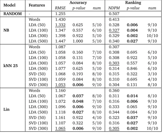
The results for the full set are shown in Table 2. For the random baseline method, we can see average NDPM value very close to 0.5, the expected value for a random ranking. It can be seen that Naïve Bayes performs worse than the two other methods. Its RMSE is worse than the random baseline, but the NDPM is better, which implies that Naïve Bayes is performing very badly as a prediction algorithm, but is still ordering the items better than chance levels. We verified that Naïve Bayes assigns the majority rating to most items. For K-Nearest
Model Features RMSE Accuracyp-value num NDPM Rankingp-value num
RANDOM - 1.255 0.507
NB
Words 1.430 0.413
LDA (50) 1.332 0.625 5/10 0.328 0.006 9/10 LDA (100) 1.347 0.557 6/10 0.327 0.004 9/10 LDA (300) 1.398 0.922 5/10 0.329 0.002 10/10 LDA (500) 1.447 1.000 5/10 0.340 0.027 9/10
kNN 25
Words 1.087 0.307
LDA (50) 1.058 0.160 7/10 0.308 0.695 6/10 LDA (100) 1.058 0.131 7/10 0.308 0.922 5/10 LDA (300) 1.057 0.084 8/10 0.303 0.557 6/10 LDA (500) 1.077 0.625 5/10 0.314 0.846 6/10 SVD (50) 1.068 0.193 8/10 0.315 0.322 3/10 SVD (100) 1.059 0.084 8/10 0.310 0.695 4/10 SVD (300) 1.053 0.006 9/10 0.304 0.131 8/10
Lin
Words 1.160 0.360
[image:9.420.80.343.15.232.2]LDA (50) 1.067 0.037 8/10 0.311 0.014 8/10 LDA (100) 1.072 0.048 7/10 0.316 0.006 9/10 LDA (300) 1.096 0.006 9/10 0.333 0.065 9/10 LDA (500) 1.118 0.027 8/10 0.344 0.084 6/10 SVD (50) 1.161 0.922 4/10 0.323 0.037 9/10 SVD (100) 1.107 0.322 5/10 0.316 0.027 9/10 SVD (300) 1.065 0.006 9/10 0.305 0.002 10/10
Table 2: Full data set performance results with random ordering (RANDOM), Naïve Bayes (NB), K-Nearest Neighbor withk=25 (kNN 25) and Regularized Linear regression (Lin). The p-value column shows the result of a Wilcoxon signed-rank test compared to the wordsmodel and statistically significant results at 0.05 are emphasized, and thenumcolumn indicates for how many users the performance improved with a topic model
[image:9.420.80.341.18.230.2]Neighbors we can see consistently good performance, which is not affected by topic-modeling or dimensionality reduction, as the small differences are not statistically significant. Regularized Linear Regression generally performs worse than kNN, except with LDA 50 and SVD 300, in which cases the results are very close to kNN. Surprisingly, for all algorithms, performance drops for LDA of higher dimension, sometimes starting at 100, sometimes at 500 features, while performance using SVD improves with higher dimension.
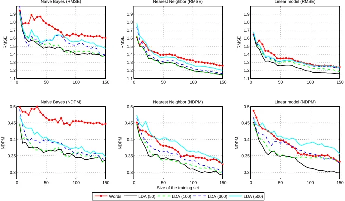
Figure 2 shows the cold-start performance for the different methods when increasing the amount of labeled data, and Table 3 shows the performance with 150 rated items. At this small amount of labeled data we can see that LDA50 gives statistically significant improvements for all methods and measures except Naïve Bayes and RMSE. We can see from figure 2, that LDA50 improves results already at much fewer than 150 ratings. At 10-20 ratings performance is better than the word-based model, being similar before that. For SVD and K-Nearest Neighbors we get improvements, but they are significant only at 300 features. In contrast, with Regularized Linear Regression SVD gives either statistically significantreductionsin performance, or statistically insignificant improvements.
6 Discussion
0 50 100 150 1.1 1.2 1.3 1.4 1.5 1.6 1.7 1.8 1.9
Naïve Bayes (RMSE)
RMSE
0 50 100 150
1.1 1.2 1.3 1.4 1.5 1.6 1.7 1.8 1.9
Nearest Neighbor (RMSE)
RMSE
0 50 100 150
0.3 0.35 0.4 0.45 0.5
Nearest Neighbor (NDPM)
NDPM
Size of the training set
0 50 100 150
1.1 1.2 1.3 1.4 1.5 1.6 1.7 1.8 1.9
Linear model (RMSE)
RMSE
0 50 100 150
0.3 0.35 0.4 0.45 0.5
Linear model (NDPM)
NDPM
0 50 100 150
0.3 0.35 0.4 0.45 0.5
Naïve Bayes (NDPM)
NDPM
[image:10.420.36.381.29.230.2]Words LDA (50) LDA (100) LDA (300) LDA (500)
Figure 2: Performances of different methods in a simple cold-start situation. On each figure the results with LDA-models along with the results with word data are shown. The upper row shows the results with RMSE and the lower row with NDPM.
Model Features RMSE Accuracyp-value num NDPM Rankingp-value num
NB
Words 1.602 0.448
LDA (50) 1.386 0.438 4/6 0.337 0.031 6/6
LDA (100) 1.384 0.563 3/6 0.338 0.063 5/6
LDA (300) 1.389 0.438 4/6 0.338 0.031 6/6
LDA (500) 1.470 1.000 2/6 0.348 0.063 5/6
kNN 25
Words 1.257 0.325
LDA (50) 1.146 0.031 6/6 0.292 0.031 6/6
LDA (100) 1.143 0.031 6/6 0.299 0.094 5/6
LDA (300) 1.159 0.031 6/6 0.300 0.031 6/6
LDA (500) 1.199 0.156 4/6 0.326 1.000 3/6
SVD (50) 1.139 0.031 6/6 0.300 0.313 4/6
SVD (100) 1.147 0.031 6/6 0.302 0.094 5/6
SVD (300) 1.162 0.031 6/6 0.293 0.031 6/6
Lin
Words 1.239 0.332
LDA (50) 1.165 0.031 6/6 0.307 0.031 6/6
LDA (100) 1.186 0.438 4/6 0.332 0.688 2/6
LDA (300) 1.229 0.313 4/6 0.328 0.688 4/6
LDA (500) 1.241 1.000 3/6 0.356 0.031 0/6
SVD (50) 1.248 1.000 3/6 0.339 0.563 3/6
SVD (100) 1.367 0.313 2/6 0.367 0.031 0/6
SVD (300) 1.158 0.031 6/6 0.302 0.094 5/6
Table 3: Cold-start data set performance results for, Naïve Bayes (NB), K-Nearest Neighbor with
k=25 (kNN 25) and Regularizes Linear Regression (Lin). The p-value column shows the result of a Wilcoxon signed-rank test compared to thewordsmodel and statistically significant results at 0.05 are emphasized, and thenumcolumn indicates for how many users the performance improved with a topic model
[image:10.420.65.357.309.498.2]performance of Regularized Linear Regression in the cold-start setting, may be because we adjust the hyperparameters for the full set. However, this can be seen as a weakness in the method, since it is very computationally demanding to optimize the hyperparameters for each data size (and user) separately. The Linear Regressor is very fast at recommendation time, requiring only one dot-product per user for each new item. The Nearest Neighbor method, in comparison, requires one dot-product calculation for each item the user has rated. However, when the number of ratings is small this is not a serious downside.
7 Conclusions
We evaluated three standard content-based recommender algorithms for a task of Finnish news recommendation. We used word counts, TF-IDF weighted word features both directly and after dimensionality reduction with SVD, and topics learned with Latent Dirichlet Allocation. We evaluated both a full data set where 10 users had 105–3891 labels each, and a cold-start data set where 6 users had 5–150 rated news items. We found that Naïve Bayes was the worst of the tested models, sometimes performing worse than a random baseline. Nearest Neighbors worked consistently well regardless of input features. Regularized Linear Regression performed well with some features, reaching similar performance as Nearest Neighbors on these features. On the full data set LDA50 and SVD300 yielded statistically significant improvements over the word features for Regularized Linear Regression, but for the other methods the improvements were not statistically significant for both measures. In the cold start simulation, we found that LDA50 yielded statistically significant improvements over the word-features for all methods. The LDA models with more than 50 topics seem to perform increasingly worse with growing amounts of topics. In contrast SVD performance improves with growing dimension, but SVD50 is worse than LDA50. These results suggest that LDA can find good features with a smaller dimension than what SVD requires, however LDA performance seems to decrease with additional topics, which can be problematic. With the amount of rated samples we have in our experiments, applying Nearest Neighbor regression is preferrable over applying Regularized Linear regression for content-based recommendation, since Nearest Neighbors is more robust, and adjusting its hyperparameterkis easier than adjusting the regularization parameters of Regularized Linear Regression.
Acknowledgments
References
Adomavicius, G. and Tuzhilin, A. (2005). Toward the next generation of recommender systems: A survey of the state-of-the-art and possible extensions. IEEE Transactions on Knowledge and Data Engineering, 17(6):734–749.
Billsus, D. and Pazzani, M. J. (2000). User modeling for adaptive news access.User Modeling and User-Adapted Interaction, 10:147–180.
Blei, D. M., Ng, A. Y., and Jordan, M. I. (2003). Latent Dirichlet Allocation.Journal of Machine Learning Research, 3:993–1022.
Cleger-Tamayo, S., Fernández-Luna, J. M., and Huete, J. F. (2012). Top-n news recommenda-tions in digital newspapers.Knowledge-Based Systems, 27(0):180 – 189.
Deerwester, S. (1988). Improving Information Retrieval with Latent Semantic Indexing. In Borgman, C. L. and Pai, E. Y. H., editors,Proceedings of the 51st ASIS Annual Meeting (ASIS ’88), volume 25, Atlanta, Georgia. American Society for Information Science.
Friedman, J. H., Hastie, T., and Tibshirani, R. (2010). Regularization paths for generalized linear models via coordinate descent.Journal of Statistical Software, 33(1):1–22.
Griffiths, T. L. and Steyvers, M. (2004). Finding scientific topics. Proceedings of the National Academy of Sciences of the United States of America, 101(Suppl 1):5228–5235.
Hoerl, A. E. and Kennard, R. W. (1970). Ridge Regression: Biased Estimation for Nonorthogonal Problems.Technometrics, 12(1):55–67.
Hofmann, T. (1999). Probabilistic latent semantic indexing. InProceedings of the 22nd annual international ACM SIGIR conference on Research and development in information retrieval, SIGIR ’99, pages 50–57, New York, NY, USA. ACM.
Lang, K. (1995). Newsweeder: Learning to filter netnews. InProceedings of the 12th Interna-tional Machine Learning Conference (ML95.
Lindén, K., Silfverberg, M., Axelson, E., Hardwick, S., and Pirinen, T. A. (2011). Hfst-framework for compiling and applying morphologies. InCommunications in Computer and Information Science, volume 100 ofSystems and Frameworks for Computational Morphology, pages 67–85. Springer.
McCallum, A. and Nigam, K. (1998). A comparison of event models for naive bayes text classification. InAAAI-98 Workshop on Learning for Text Categorization, pages 41–48. AAAI Press.
Mooney, R. J. and Roy, L. (2000). Content-based book recommending using learning for text categorization. InProceedings of the Fifth ACM Conference on Digital Libraries, pages 195–204. ACM Press.
Rashid, A. M., Karypis, G., and Riedl, J. (2008). Learning preferences of new users in recommender systems: an information theoretic approach.SIGKDD Explor. Newsl., 10(2):90– 100.
Salton, G. (1989). Automatic text processing: the transformation, analysis, and retrieval of information by computer. Addison-Wesley Longman Publishing Co., Inc., Boston, MA, USA. Schein, A. I., Popescul, A., Ungar, L. H., and Pennock, D. M. (2002). Methods and metrics for cold-start recommendations. InProceedings of the 25th annual international ACM SIGIR conference on Research and development in information retrieval, SIGIR ’02, pages 253–260, New York, NY, USA. ACM.
Takács, G. and Tikk, D. (2012). Alternating least squares for personalized ranking. In
Proceedings of the sixth ACM conference on Recommender systems, RecSys ’12, pages 83–90, New York, NY, USA. ACM.
Wilcoxon, F. (1945). Individual Comparisons by Ranking Methods. Biometrics Bulletin, 1(6):80–83.
Yao, Y. Y. (1995). Measuring retrieval effectiveness based on user preference of documents. J. Am. Soc. Inf. Sci., 46(2):133–145.