Colour image quantisation and coding for optimal perception

(1)

University of Warwick institutional repository:http://go.warwick.ac.uk/wrap A Thesis Submitted for the Degree of PhD at the University of Warwick

http://go.warwick.ac.uk/wrap/73515

This thesis is made available online and is protected by original copyright. Please scroll down to view the document itself.

(2)

Colour Image Quantisation and Coding For Optimal Perception

Roderick William McColl, BSc(Hons), MSEE

A thesis submitted to The University of Warwick

for the degree of Doctor of Philosophy

(3)

Abstract

Once a digital image is processed in some way and the reconstruction is compared to the original, the final arbiter of reconstruction quality is the human to whom the images are presented. The research presented here is concerned with the development of schemes for the quantisation of colour images and for the encoding of colour images for transmission, with the goal of minimising the perceived image distortion rather than minimising a traditional error signal statistic.

In order to quantise colour images with minimum perceived distortion, a colour space is sought in which Euclidean distances correspond linearly to perceived colour difference. The response of the visual system to colour and colour difference is investigated. A new quantisation scheme is developed and implemented to achieve a colour image compression ratio of approximately 6: 1. Three variations on the basic quantiser algorithm are considered and results of applying each variation to three test images are presented.

Two-component encoding of colour images for low bit-rate transmission is investigated. A new method of encoding the contents of the image regions following contour extraction is developed. Rather than using parametric surface descriptions, a quad-tree is constructed and a simple measure of perceived image contrast threshold is used to determine the transmitted data. Arithmetic entropy coding is used to discard statistical redundancy in the signal. A colour wash process recreates the colour in each region. Implementation details are presented and several examples are given to illustrate differing contrast thresholds with compression rates of up to 50: 1.

(4)

List of Contents

Chapter 1. Introduction 1

1.1. Theories of Vision 1

1.2. Colour Standards 4

1.3. Colour Spaces 6

1.4. Image Processing 9

1.5. Image Distortion 11

1.6. Other Chapter Contents 12

Chapter 2. Quantisation of Colour Image Data 14

2.1. Introduction 15

2.2. Colour Space Transformations 16

2.3. MacAdam's Geodesic

.

19

2.4. Quantisation Parameters 29

2.5. Quantisation by Data Clustering 33

2.6. The "k-means" Test 34

2.7. Quantiser Colour Space Conversions 36

2.8. Quantisation of Achromatic Data 39

2.9. Quantiser Implementation Details 40

2.10. Sources of Quantiser Error

.

42

(5)

2.12. Three Variations on the Quantiser Algorithm 2.13. Discussion of Results

2.14. Summary

Chapter 3. Two-Component Colour Image Coding 3.1. Introduction

3.2. Discussion of Image Models .

3.3. The Quad-Tree - Motivation and Use 3.4. The Use of Incomplete Quad-Trees . 3.5. Coding the Quad-Tree Data .

3.6. Coding the Chromatic Content of the Region 3.7. Threshold Coding of Quad-Tree Data - Image

Contrast

3.8. Entropy Coding 3.9. Arithmetic Coding

3.10. The Binary Arithmetic Coder and Q-Coder . 3.11. Region Coding - Quantisation

3.12. Discussion of the Coding Process 3.13. Decoding the Compressed Data 3.14. Edge Reconstruction .

3.15. Smoothing of Quad-Tree Aliasing

(6)

3.16. Test Results with Varying Compression and Reconstruction Quality

3.17. Summary

Chapter 4. Textures - Analysis and Synthesis

4.1. Texture Models - Statistical and Structural . 4.1.1. Statistical Models

4.1.2. Structural Models

4.2. Two Recent Approaches to Texture Synthesis 4.3. Texture Synthesis for Colour Data Compression 4.4. The Autocorrelation Function as an Estimator 4.5. Autocorrelation Estimates from Image Regions 4.6. Multiple Autocorrelations for Texture Synthesis 4.7. Texture Primitive and Placement Rules

4.8. Test Results

4.9. Bilinear Interpolation for Improved Texture Synthesis

4.10. Cost Comparison of Region Compression Schemes 4.11. Texture Synthesis from Spectral Magnitudes 4.12. Summary

Chapter 5. Conclusions

(7)

5.l. Summary of Chapter 2 - Quantisation of Colour Image Data

5.2. Summary of Chapter 3 - Two-Component Colour Image Coding

5.3. Summary of Chapter 4 - Textures: Analysis and Synthesis

5.4. Distortion Measure - The MSE and Human Perception

5.5. Sensitivity to Luminance - Logarithmic Relationships .

5.6. The "Just Noticeable Contrast Difference" Threshold

5.7. Texture Synthesis - Further Developments 5.8. The Role of the Chromatic Component 5.9. Video Communications in the 1990s

References

Appendix A. Details of Experimental Viewing Conditions and Generation of the Colour Prints

(8)

List of Figures

Figure 1.1. CIE colour matching functions for the Standard Observer

Figure 2.1. MacAdam's ellipses plotted on CIE x-y chromaticity chart

Figure 2.2. MacAdam's ellipses plotted on CIE-UCS chart. Figure 2.3. MacAdam's ellipses plotted on geodesic

chromaticity chart

Figure 2.4. Plot of CIE x- and y-Ioci on MacAdam's geodesic chromaticity chart

Figure 2.5. Chromaticity locus of colour image in figure 2.9 plotted on r-g chromaticity chart.

Figure 2.6. Chromaticity locus of figure 2.9 plotted on CIE x-y chromaticity chart

Figure 2.7. Chromaticity locus of figure 2.9 plotted on CIE-UCS u-v chromaticity chart

Figure 2.8. Chromaticity locus of figure 2.9 plotted on MacAdam's geodesic chromaticity chart Figure 2.9. Colour image used for chromaticity plots

(colour print) .

(9)

Figure 2.10. Typical colour gamut and r-g chromaticity

axes plotted on CIE x-y chromaticity chart 31 Figure 2.11. Colour gamut from figure 2.10 plotted on

MacAdam's geodesic chromaticity chart 32 Figure 2.12. Quantisation flow diagram featuring Transmitter

(fx) and Receiver (Rx) elements 44 Figure 2.13. Pixel arrangement at reconstruction 46

Figure 2.14. Original digitised frame from video codec

test sequence "Miss America" (colour print) 49 Figure 2.15. Original digitised frame from video codec

test sequence "Split Screen" (colour print) 50 Figure 2.16. Original digitised frame from video codec

test sequence "Trevor White" (colour print) 51 Figure 2.17. Quantisation performed on frame "Miss America"

using quantiser Method I (colour print) 53 Figure 2.18. Quantisation performed on frame "Split Screen"

using quantiser Method I (colour print) 54 Figure 2.19. Quantisation performed on frame "Trevor White"

using quantiser Method I (colour print) 55 Figure 2.20. Quantisation performed on frame "Miss America"

(10)

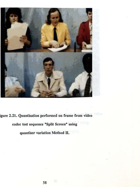
Figure 2.21. Quantisation performed on frame "Split Screen II using quantiser Method II (colour print)

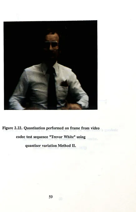
Figure 2.22. Quantisation performed on frame "Trevor White" using quantiser Method II (colour print)

Figure 2.23. Variation of the maximum area on MacAdam's geodesic chromaticity chart as luminance values varies

.

Figure 2.24. 3D plot of available chromaticities on MacAdam's geodesic chromaticity chart as luminance varies Figure 2.25. Plot of the intersection of luminance planes

through the RGB colour cube

Figure 2.26. Quantisation performed on "Miss America II using quantiser Method III (colour print) Figure 2.27. Quantisation performed on "Split Screenll

using quantiser Method III (colour print) Figure 2.28. Quantisation performed on "Trevor White"

using quantiser Method III (colour print)

Figure 3.1. Region taken from a segmented frame in the test sequence "Miss America" (colour print) Figure 3.2. Region taken from a segmented frame in the

test sequence "Trevor White" (colour print)

(11)

Figure 3.3. Dimensions of highly convoluted region taken from

segmented frame in test sequence "Trevor White" 82 Figure 3.4. Centred quad-tree over region at various

resolutions 83

Figure 3.5. Visual contrast sensitivity curves as a function

of spatial frequency

.

90

Figure 3.6. Example of arithmetic coding for three-symbol

alphabet 95

Figure 3.7. Distribution of Parent-Child Differences for all

quad-trees constructed from frame "Miss America" 100 Figure 3.8. Distribution of Parent-Child Differences for all

quad-trees constructed from frame "Split Screen" 101 Figure 3.9. Distribution of Parent-Child Differences for all

quad-trees constructed from frame "Trevor White" 102 Figure 3.10. Flow diagram of the region coding algorithm 106 Figure 3. 11. Illustration of phantom nodes in the quad-tree and

their assignment in the upward averaging process 111 Figure 3.12. Illustration of the role of phantom nodes in the

downward interpolation process 112

Figure 3.13. Flow diagram of the decoder algorithm 115 Figure 3.14. Original digitised frame from test sequence

(12)

Figure 3.15. Original digitised frame from test sequence

"Split Screen" used for codec (colour print) 117

Figure 3. 16. Original digitised frame from test sequence

"Trevor White" used for codec (colour print) 118 Figure 3.17. Edge map computed for frame "Miss America" 119 Figure 3.18. Edge map computed for frame "Split Screen" 120

Figure 3.19. Edge map computed for frame "Trevor White" 121

Figure 3.20. Reconstructed frame from sequence "Miss America"

with c

=

0.06 (colour print) 123

with c

=

with c

=

Figure 3.23. Reconstructed frame from sequence "Split Screen"

with c

=

with c

=

with c

=

Figure 3.26. Reconstructed frame from sequence "Trevor White"

(13)

with c = 0.10 (colour print)

with c = 0.12 (colour print)

Figure 4.1. Diagrams of the various stages in the texture

identification and extraction of placement rules for a region in the image

Figure 4.2. Examples of the placement rules according to repetition vectors extracted from texture analysis

Figure 4.3. Relationship of pixel in synthesised region to pixel

found in the texture primitive rectangle

Figure 4.4. Original frame from test sequence "Trevor White" (colour print) .

Figure 4.5. Synthesised textures using input from figure 4.4

(colour print) .

Figure 4.6. Segmentation map of original frame, with synthesised regions shown shaded

Figure 4.7. Illustration of the bilinear interpolation algorithm

Figure 4.8. Synthesised textures with bilinear interpolation

in each region to provide variation of mean

intensity level (colour print) .

(14)

[image:14.481.42.460.0.797.2]

Figure 4.9. Segmentation map, highlighting two

(15)

List of Tables

Table 2.1.

Table 2.2.

Table 3.1.

Table 4.1.

Chromaticity Mean Square Error for quantisation Methods I, IT and ITI .

Chromaticity Mean Absolute Error for quantisation Methods I, IT and lIT .

Region Coder statistics for various contrast threshold values

Comparisons of approximate coding cost for texture synthesis of the two regions highlighted in figure 4.9 and for the entropy-coded output from the quad-tree coder used in chapter three

67

68

122

(16)

Declaration

I hereby declare that, except where specifically acknowledged, all work presented in this thesis was carried out by me, Roderick William McColl, and that it has not been submitted elsewhere for the purpose of obtaining an academic

(17)

Acknowledgements

There are a number of individuals to whom I would like to express my deepest gratitude. I thank my supervisor, Dr. Graham Martin, for his considerable help both during my years at Warwick and also during the period of writing and submitting the thesis from Texas. Dr. Roland Wilson gave me much technical advice on image coding; my fellow students (now Drs.) Andrew Calway

and Martin Todd also provided many valuable suggestions. My colleagues at GEC Hirst Research Centre, Dr. Vaughan Stanger and Ms. Alexandra Symons, involved me in many helpful discussions. Finally I thank my parents who have always encouraged me to complete whatever academic endeavour I start.

(18)

Chapter 1. Introduction

This thesis concentrates on aspects of colour image quantisation, redundancy and coding, and how the pertinent factors may be manipulated within the context of minimising the perception of noise or errors by the average viewer

of processed images; by using perceptual criteria, any processed image should contain an "optimal" distortion, i.e. one that is least easily perceived, hence the thesis title. The investigation of these factors includes visits to the fields of human physiology, colour science, optical physics, image processing and information theory. The primary motivation in the investigation is the considerably increased raw storage requirement of typical colour images compared with their grey-scale counterparts, and the likely impact of successful compression of the image beyond that which is currently considered acceptable. A specific application for such compression would be video conferencing at the increasingly available ISDN (64kbitls x N) bandwidths.

1.1. Theories of Vision

(19)

this theory was proposed in 1807 by Thomas Young [1] and elaborated by von Helmholtz [2] a half century later (see MacAdam [3] for evidence to the contrary.) Young assumed that the eye contains three independent response mechanisms to light: one predominantly sensitive to the shorter wavelengths of light, the second favouring the middle part of the visible spectrum and the third most sensitive to the longer wavelengths. Each of these responses would have some value over the whole visible spectrum, and the visual sensation to a given light source would come from the integration of the three responses with the components of the light. In 1860 Maxwell determined the shape of three responses from experimental observations [4] (a reprint of Maxwell's paper can be found in MacAdam [5]). Maxwell's experiment is widely considered to be the first fundamental study of colour vision. His experiment involved the arbitrary choice of three spectral wavelengths or primaries, from which light of any wavelength or wavelengths could be generated, and subsequently matched, or

distinguished, by the receptors of the eye. These primaries can be labelled "red", "green" and "blue" according to the subjective appearance of monochromatic light of the selected primary wavelengths. Maxwell selected the primary wavelengths to be 630 nm for the red primary, 528 nm for the green primary and 457 nm for the blue primary. These colour receptors in the retina are named "cones", because of their physical appearance.

(20)

alternative theories for colour VISIon lay in the way the previous models

performed in the case of abnormal colour vision, such as colour blindness. The

theory did not adequately account for the sensations experienced by dichromats,

the most common of which is the inability to distinguish between red and green. Konig [6] suggested that one of the colour receptors in the eye may actually

perceive brightness only, i.e possessed an achromatic response, with the other

two mechanisms providing the chromatic response. Hering [7] proposed a theory

based on these ideas in 1878, known as the

opponent-colours

theory. The theory states that the sensation of colour is a result of three opposing pairs of processes: a light-dark, a red-green and a yellow-blue. From a physiological standpoint, this

theory allowed for dichromatic vision simply by the notion of the loss of one of these processes. Unfortunately, the advantage in Young's theory was that it was

simple and deemed physiologically plausible, whereas Hering's theory was considered unacceptable physiologically.

The logical progression from these early theories were more complex

models of colour vision which included parts of both trichromacy and

opponent-colours [4]. These are known as

stage

theories because they incorporate one or more distinct transformations of the processes in the visual system, from the retina to the optic nerve. The stages began with a retinal process similar to that

suggested by Young, ending with a signal similar to an opponent-colours process.

(21)

undertaken to provide a quantitative account of opponent-colours processes. Although Young's cone theory has always been generally accepted, however, it was not until the latter part of this century that any physical evidence for such responses appeared in the literature [8].

1.2. Colour Standards

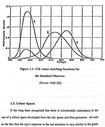
As the science of colour vision developed, many researchers contributed their own models, each differing slightly in an attempt to account for those situations in which other models failed. In order to provide some sort of international standard, in 1931, the Commission Internationale de l'Eclairage (CIE) [9] defined the colour response curves for the eye of the Standard

Observer, a normal male trichromat (in fact an average of previous experiments by Wright [10] and Guild [11]), in terms of spectrum primaries of 600 nm, 546 nm and 436 nm, considered to be a better choice of primaries from a physiological standpoint. These curves have been used to specify paints, television monitors, etc. from the view of how colours appear to a normal human. These curves are shown in figure 1.1 (from Judd [4]). It is apparent that the range of light that the human visual system can perceive is about 380 to 700 nm.

(22)

that volume occupied by all possible colour vectors with axes drawn from the three selected primaries. One of the disadvantages of the normal colour matching functions using the red, green and blue primary wavelengths, is that in certain situations, negative amounts of one or more primaries are required to generate the desired colour [4]. Obviously there can be no such thing as a negative amount of radiant flux; however, the concept is well understood to mean that some amount of one of the primaries is subtracted from the light incident on the retina in order to make the colour match (this is one of the central concepts in the laws of Grassman for compound colours [12]). However, since an additive colour system is a requirement for the likes of colour display systems such as televisions, the

CIE established a colour space in which all colours that can be seen are composed of positive amounts of the three primaries. This colour space is referred to as the (CIE) XYZ colour space [9], and it contains what is known as the cone of realisable colours.

A more common representation of vectors in the CIE colour space is the specification of the chromaticity of a colour, which, together with a third value, the luminance, (Y), provide a direction and magnitude from the origin. Working with a 2-dimensional chromaticity space makes the graphical display of graphical colour information more straightforward, and also provides a dimensionless, normalised, reference for the spectrum, which resolves the extreme changes in

(23)

2.0----~----~----~----.---~----~----~---,---,

t.,~--~~r-~~--~----~----~---;----~---+----~

O.4~--~----~----~+---~~--~----~~~~---+----~

~&O~~~--~~~=6~O--~~~~~--~~~e-O----.~2~O--~~~~7~OO~--~'.0

[image:23.504.46.482.73.598.2]

A(mp)

Figure 1.1. CIE colour matching functions for the Standard Observer.

(Source: Judd [4]).

1.3. Colour Spaces

(24)

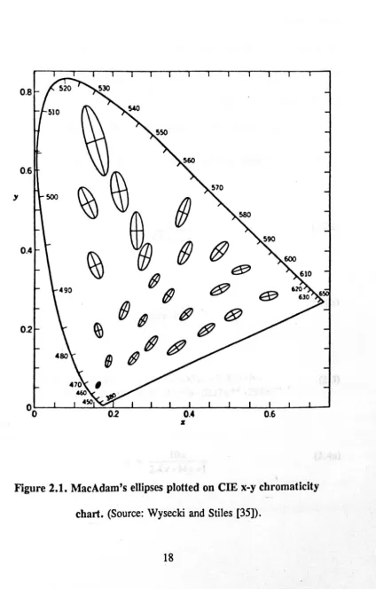
difference perceived by the observer is not isotropic. The colour space is not

metric from the viewpoint of sensed changes. The importance of a metric colour space to the printing industry has driven research to find such a colour space for

many years. MacAdam, however, has shown that a truly metric colour space is impossible to attain in 3 dimensions [13], although he and others have presented

approximations to it based on curve fitting experiments. The experiments

conducted by MacAdam and others in measuring the responses of a number of

observers to changes in the chromatic content of equiluminous light sources and

their perceptions of just noticeable differences in colours, led to a transformation under which the plot of just noticeable differences on the 2-d chromaticity

diagram produced circles. Plotting within the CIE (x,y) chromaticity space or the

(r,g) chromaticity space show ellipses, with longer axes in the direction of the

green and red primaries. MacAdam was unsuccessful in getting the CIE to adopt

his geodesic chromaticity model [14], so called because the curve between any

two colours on the chromaticity diagram is a straight line, or geodesic, and

involves the least number of colour differences. However the CIE in 1961 adopted his recommendations for a more metric space than the XYZ colour space,

labelled the UVW colour space [15]. Transformations from RGB to XYZ and to

UVW can all be achieved through matrix multiplication.

(25)

which was conceived by the artist Edward Munsell in 1905 as an attempt to bring

a rigourous language to the description of colours. The Munsell Colour

Company's tables of colour tiles are used extensively in the colour industry today.

During the 1950s and 196Os, Hurvich and Jameson conducted a number

of investigations within the framework of an opponent-colours theory [19]. Their argument for this model was that an enormous amount of research had been

expended in finding the "best" set of primary wavelengths under a Young model, with no general consensus emerging as to the "right" choice, because of the

failure of the model to account for all the facts of colour vision. Their work

yielded fundamental quantitative models whereas, before, the data were decidedly qUalitative. In fact, their model was a two-stage model, incorporating a

trichromatic "front end" to the visual system with response curves similar·to that

of the CIE standard observer, and an appropriate transformation to yield the

light-dark, red-green and yellow-blue sensations which are transmitted along the

optic nerve. They stated that physiologically, this model made excellent sense because it explained, in a simple fashion, phenomena such as chromatic

adaptation and colour constancy, for which the three colours theories failed to

provide. Ohta et al. [20] also propose, from empirical observations, an

opponent-colours model in which three best-fit colour response functions are used to

(26)

The opponent-colours theory is of interest because the implication is that the visual system performs its own colour compression [21], as the red, green and blue responses from the cones in the eye are transformed into a space with three pathways which contain high-bandwidth information (the light-dark sensation), medium-bandwidth information (the red-green sensation) and

low-bandwidth information (the yellow-blue sensation). In recent years, many advances in image processing have been made by considering human physiology and attempting to exploit its weaknesses, rather than generating ad hoc models and algorithms. It seems to make sense, then, to base investigations of colour image properties on considerations of the characteristics of the visual system, since that is the intended "receiver".

1.4. Image Processing

There are many examples in the literature of quantisation schemes for colour image data. Since the work of Max on quantisation with a minimum mean-square error criterion [22], and the subsequent work of Linde, Buzo and

(27)

Limb et al. [26] does discuss this issue.

Image processmg has evolved rapidly as a science throughout its reasonably brief history. The main stumbling block to applications has been the sheer data throughput required when developing and testing algorithms, a problem which has only recently eased with the development of inexpensive, fast computer technology. Two distinct generations of image processing algorithms have been reported in the literature [27]. The so-called first generation includes both spatial and transform techniques, for instance DPCM and DCT algorithms, both of which have been extensively represented in the literature, but the majority of algorithms have at best assumed that colour image processing is no more than an extension of gray-scale processing, with the two chromatic channels simply being assumed to occupy narrower bandwidths than the achromatic signal, but possessing similar properties.

(28)

at differing resolutions. Texture coding schemes attempt to find simple base

patterns which can be repeated throughout a region of the image to synthesise the original. The model which has been investigated in this research is known as the

region-growing

model. The model assumes that the average scene or image

frame, is composed of large areas or regions in which the data is stationary and

in which the variation in pixel value or values is small. These regions are

bounded by discontinuities, known as edges, where there are abrupt changes in

the image content. The processing of the two feature types involves encoding the

edge pixels and finding succinct descriptions of the slowly changing information

in the regions. The human visual system is known to be far more sensitive to

discontinuities in image content than to slowly changing properties, and the expected compression from this type of coding scheme is potentially enormous.

1.5. Image Distortion

Another area of interest within this investigation has been the

determination of a suitable error measure for the results of image processing

algorithms. The traditional mean-square error estimate is widely agreed to be a

poor representative of the success of any image compression scheme [26,29,30], simply because it is physiologically unacceptable, requiring the visual system to

(29)

not in another with the same measure. Referring to the last paragraph, it is known that the visual system is far more sensitive to sharp changes in an image than to low spatial-frequency ones. An ability to estimate the impact of a small number of large errors within a processed image must be taken into account. This thesis includes analyses of the applicability of error measures to the success of colour image quantisation and coding schemes with a view to providing substantial

agreement between subjective appearance and numerical error value.

1.6. Other Chapter Contents

The next chapter contains an investigation of colour quantisation for minimum perceived distortion, with a further description of the colour space and chromaticity space, colour space homogeneity, linearity and metricity. Quantisation schemes which are found in the literature are discussed. A novel quantisation is developed, along. with complete details of an implementation. Results are obtained from three test images, together with a discussion of error statistics. A comparison of the success of the algorithms developed in this chapter

with selected other literature is also given . .

(30)

a brief presentation of the methods used to generate the edges and regions which make up each image frame. The rest of the chapter is devoted to an investigation of models for coding colour regions and their applicability within the framework of the human visual system. The details of a new region-coding model are presented, along with an investigation of arithmetic entropy-coding schemes for

further compression of the region descriptions. Implementation details and results are presented in depth, and comparisons are made with other literature.

Chapter four is concerned with the analysis and synthesis of the textures which can be identified in colour images, and the potential for compression based on popular texture models in the literature. An algorithm is developed to improve the compression achieved in chapter three on certain colour image regions containing a feature which is regularly or semi-regularly repeated; the synthesis of such features and the rules for repetition are derived and a comparison is made between cost and perceived quality of reconstructed regions using the algorithms developed in this chapter and in the previous one.

(31)

Chapter 2. Quantisation of Colour Image Data

Consider the storage requirements for a typical digitised colour image. The

matrix size is usually 256x256 pixels at low resolution, and perhaps 512x512

pixels for a high-quality image (most television standards offer resolutions in the

500-600 line range). If the data are stored as RGB triplets, the typical

quantisation is to 8-bits per primary, 24-bits per pixel, or 24 bpp. Therefore, for

a high-resolution digitised colour image, the requirement is 786432 bytes, or

three-quarters of a MegaByte. Even in the days of inexpensive magnetic media, a sequence of such images requires a considerable storage commitment, and

access to anyone frame or pixel for real-time applications requires high-speed

disk access hardware. Given that the human observer is incapable of

distinguishing the 16.7 million colours available at 24-bpp, it is often desirable

to provide quantisation to considerably reduce the storage cost per frame,

depending on the application envisaged for the data.

In this chapter, we will investigate an algorithm, designed to find the quantisation of any colour image such that any introduced distortion in the

reconstructed image is always the least easily perceived. Three variations on a

(32)

reconstructed images, and an attempt is made to quantitatively measure the distortion, if any, that is introduced by the quantisation process. The main interest is in reducing as far as possible the cost of storing the chromatic content of the colour image. The results are favourable when compared with those found elsewhere in the literature.

2.1. Introduction

Since the early 1970s, there has been interest in processing colour images as well as monochromatic ("black-and-white") images. Quantisation of the image

(33)

demonstrated an agreement between subjective measurements of introduced colour

image distortions with MSE m,easurements for the distorted images. He did not attempt any quantisation experiments, however. Stenger [32] considered the

perception of chrominance differences in his design for a quantiser of television

signals. He computed a number of luminance-dependent grids to quantise the

signal. Kurz [17] used a similar scheme and incorporated the MacAdam geodesic

as a quantisation grid for pixel chromaticities, rather than the chrominance

considered by Stenger. Multiple grids were used depending on the quanti sed

luminance value. Many schemes which have become popular, however, such as

those of Heckbert [33], and Lena and Mitchell [34], which work by repeatedly

dividing the histogram of the data into blocks, depend solely on the use of the

RGB colour space for their algorithms. Given that, in most natural scenes, the

colours are generally unsaturated [26], then the correlation between the red, green

and blue components will be high. The effect of a linear transformation to a more

uncorrelated set of primaries may itself be sufficient to quantise the image in some cases. (It should be mentioned that in the field of computer graphics,

images often contain artificially saturated colours.)

2.2. Colour Space Transformations

The aim of this study is to quantise the image in such a way as to provide

(34)

interest is not in finding, on a pixel-by-pixel basis, the smallest difference

between the input primaries - red, green and blue - and the output. Consider the

diagram shown in figure 2.1. It is a plot of some experimental results obtained

by MacAdam (from Wysecki and Stiles [35]), which show the ellipses of just

noticeable differences about some 25 different chromaticities, plotted on the CIE

(x-y) chromaticity chart [9]. The circumferences of each ellipse indicate the

distance travelled on the chart from the ellipse center before the observer noticed,

on average, a definite change in the displayed colour. It is apparent that human

perception of chromaticity change is not linearly related to the

cm

co-ordinate

system. Since the CIE XYZ colour space is linearly related to the RGB colour

space in which the display hardware operates, attempting to minimise the

differences between input and output of RGB triplets is not guaranteed to provide

the closest colour match as far as the average observer is concerned. The diagram

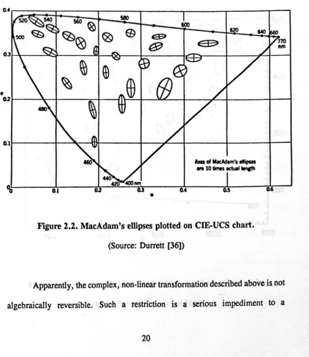
in figure 2.2 (from Durrett [36]) shows these same ellipses plotted on the

CIE-UCS (u-v) chart [15], a linear modification of the x-y chart. There is a

visible improvement, but the radii of the ellipses still vary considerably. There

is considerable ongoing research aimed at providing a linear transformation of the

x-y chart which aproximates circles rather than ellipses (although exactly

equal-radii circles cannot be generated this way [13]). The importance of the linear

requirement is that without it, the centre-of-gravity principle (which defines the

chromaticity of a two colour mixture as the luminance-weighted average of the

(35)

become unpredictable [26].

0.6

y 500

(J

0.4

~ ~

@@

&J

@@

~

@

G

~

@

0.2

~

IJ

t!P

[image:35.510.64.489.105.770.2]

m

G

Figure 2.1. MacAdam's ellipses plotted on

eIE

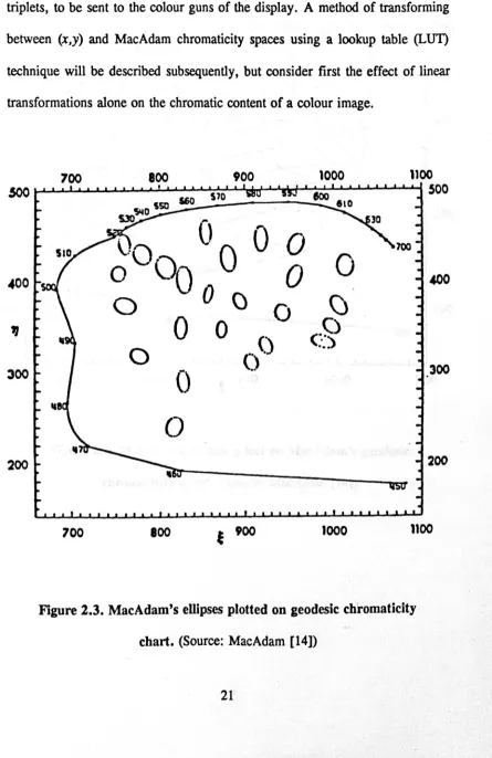
x-y chromaticity

(36)

2.3. MacAdam's Geodesic

MacAdam [14], allowing for the loss of centre-of-gravity, has generated a pair of non-linear transforms which generate the almost circular ellipses shown in figure 2.3 (from MacAdam [14]). The resulting chart is called a geodesic, because the straight-line distance from one point to any other on the chart involves the least number of

just noticeable

colour

differences

Gnds). The two equations which MacAdam derived by experiment are (from [14])

T)

=

404b-185b2+52b3+69(1-b~-3a2b+30ab3 , (2.1)

where

lOx _(2.2a)

a

=

4.2y-x+1

and

b

=

lOy

(2.2b)

4.2y-x+1

~ = 3571a'-lOa4-520b'+13295b3+32327ab- (2.3) 25491 alb -41672ab2 + lOa3b -5227 a1!2 +295 al/4 ,

where

lOx

a = - - - - (2.4a)

2.4x+34y+l

(37)

b = _ _ lO-:!.y _ _ 2.4x +34y + 1

(2.4b)

Of course, the symbols

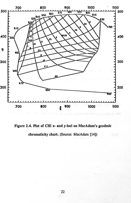
x

and y denote the CIE chromaticity co-ordinates, Figure

2.4 (from MacAdam [14]) illustrates the relationship between the CIE and MacAdam domains for loci of

x

and

y,

•

_{~~--~~+---~+-~~-+--~~-+----~-+---+--~}

~1~---+-~~-tt&---+-~~--+---4---4-~

0.1

•

G.4

[image:37.508.43.493.236.756.2]

Alles of MacAdam', tIIipsa . . 10 times IduII ~

Figure 2.2. MacAdam's ellipses plotted on C~UCS chart. (Source: Durrett [36])

G.6

(38)

quantisation scheme, since it is a requirement that the output data are RGB

triplets, to be sent to the colour guns of the display. A method of transforming

between (x,y) and MacAdam chromaticity spaces using a lookup table (LU1)

technique will be described subsequently, but consider first the effect of linear

transformations alone on the chromatic content of a colour image.

700 800 900 1000 1100

500 • 500

S60 5'0 ,..

.

II

0

700

\'''0

·0

₀

o

00

0

400

o

0 ()

0 C)

o

0 ()

(.9

0 ₍₎

:

.:>

300

()

..

0

200 200

[image:38.504.47.492.93.779.2]

700 800

E

900 1000 1100

Figure 2.3. MacAdam's ellipses plotted on geodesic chromaticity

(39)

700

1000

1100

500~~~~~~~~~~~~~~~~~~~~~~~500 800

900

AOO AOO

fJ

300 300

200

[image:39.508.43.487.79.765.2]

700

800

1000

1100

Figure 2.4. Plot of eIE x- and y-Ioci on MacAdam's geodesic

chromaticity chart.

(Source:

MacAdam [14])

(40)

Figures 2.5, 2.6, 2.7 and 2.8 indicate the extent of some chromaticity diagrams occupied by the data (at all luminance levels) from the image shown in figure 2.9. The change in the size of the area represents a transfer of image energy from the red, green and blue primaries to the luminance primary. Figure 2.5 is plotted from the r-g chromaticity space, using the normalisations

R

r =

-R+G+B

G g=

-R+G+B

(2.5)

where R, G and B are values for the pixel, usually in the range 0-255, i.e. 8-bit quantities. It is assumed that any gamma correction which has been applied to these prior to use has been equalised.

The axes of figure 2.6 are the CIE 1931 (x,y) chromaticity axes. Those of figure 2.7 are the CIE 1960 DCS (u, v) space, related to the (x,y) space by the following transforms (from [15]):

4x

u

=

--2x+12y+3

v = _ _ 6~y __ -2x+12y+3

(41)

1.0

o

r

Figure 2.S •

.

Chromaticity locus of colour image in figure 2.9

plotted on r-g chromaticity chart.

(42)

y

o

_x

Figure

2.6.

Chromaticity locus of figure

2.9

plotted on

em

x-y chromaticity chart.

(43)

1.

u

Figure

2.7.

Chromaticity locus of figure

2.9

plotted on

CIE-UCS u-v chromaticity chart.

(44)

500T---~

140 660

Figure 2.S. Chromaticity locus of figure 2.9 plotted on

MacAdam's geodesic chromaticity chart.

(45)

Figure 2.8 is a plot in the MacAdam geodesic. In all of the

transformations, the lightness co-ordinate, which will be referred to from now on

as the grey-level, or the intensity, or the luminance, of the colour, is related to

the red, green and blue values by the standard (CIE) formula (normalised to a

particular distribution of light known as illuminant C)

Y

=

0.299R +0.587 G +0.114B (2.7)

This formula represents the response of the standard observer to provide a match

to an equal-intensity light of any mixture of wavelengths.

Figure 2.9. Colour image used for chromaticity plots in figures 2.5,

2.6, 2.7 and 2.8.

(46)

2.4. Quantisation Parameters

From the previous figures, then, it is apparent that simply transforming from RGB to one of the chromaticity-luminance spaces seems to provide a

considerable compression of the "colour" in the image. At this point, some

consideration should be given as to how coarse a quantisation, i.e. how many

bits-per-pixel, is likely to be acceptable. It is widely held, for instance, that the

untrained eye is only capable of discriminating about 64 grey shades, or 6 bits.

What about chromaticity? Consider figure 2.8 and Maxwell's geodesic once

again. The ellipses in the geodesic, which indicate typical ability to perceive

colour difference, indicate that about 10 units in the geodesic correspond to ajnd.

Hence, under the assumption that one can add these across the chart, figure 2.8

shows that about 4 bits are needed to adequately represent the typical image. But

to provide a finer quantisation scheme, consider figure 2.10. (from Fink [37]).

This figure shows the (x,y) chart with the typical gamut or extent of realisable colours contained inside the triangle. Notice that the true range of colours lies

within the triangle with sides defined approximately by the following ineqUalities:

0.14~~0.66; 0.07 ~y~0.72; y~O.Sx; x+y~1.0 (2.8)

Plotting this triangle on the geodesic generates the relationship shown in figure

2.11. The range of realisable colours is reduced to an area bounded by the

(47)

720~~:d04O; 240~t'\~480 (2.9)

Note that MacAdam's experimental results indicated a threshold of at least

10 units on his chart before a colour change was detected on average. With this

information, it should be reasonable to halve the resolution of the space as a

quantisation, without loss of information. This will be discussed further when the

design for the LUT is presented.

Returning to the discussion of perceived distortion, it is apparent that

MacAdam's chart is a metric space, because straight line vectors correspond to

the smallest amount of perceived equiluminous colour change. The nature of this

space allows an analytic measure of colour distortion, in that the distance between

any two points on the chart is linearly related to the perceived difference, a

feature known as

proportionality,

and the perceived difference is independent of the absolute positions of the points, a feature known as

homogeneity.

In fact, it

is now meaningful for us to apply a simple measure like the Mean Square Error

(MSE) measure,

(2.10)

to the quanti sed pixel chromaticity values, and thus provide a reasonable account

of the average distortion perceived by the viewer. At this point, it should be

(48)

not been explored. This will be discussed in future sections.

0.9~--~----'---'---~----~----~--~r----'

0.8 1--;IL..--+--.:!IIoo.c:---t----~-- ----r---+---I

0.71f---t-0.61---+----t---+~~T--I_-_+--_+_-_t

500

>- 0.5 H----+----~_+_--t---~~~_"k:

OA~---+---+~----r---_+----,_~~~~~----~

610

Q3 --~~--~----~----+-~~~~~630 620

640

700-780

0.1 J---il:-i~~- ~--,;t'~--_t----_+_---+_--_1

0.3 0.4

I

0.5 0.6 0.7 0.8

Figure 2.10. Typical colour gamut (Solid) and r-g chromaticity (Dotted)

plotted on CIE x-y chromaticity chart. Point "C" corresponds to

(49)

800 900 1000 1100

.500 J-L-L-'-I.-I.."jL-I..I~L,..&...I~L-I..IL.L.IL..&..I!~~~---""~~~""""".I.-L...I..A...&..&..IL..(

500

AOO

300

200

700

100

1000 1100

Figure 2.11. Colour gamut from figure 2.10 plotted on MacAdam's

geodesic chromaticity chart. "r", "g" and "b" arrows correspond

to "RED", "GREEN" and "BLUE" in figure 2.10.

Having considered the various colour spaces in which perceived distortion

closely matches distance through the space, and the use of measurements of such

distortion, the discussion turns to the implementation of an image quantisation

scheme. The goal, which was somewhat arbitrarily chosen, is to reproduce 24

(50)

quantisation scheme would thus provide approximately twice the compression of

common schemes with less visible distortion. Before the details of the proposed

scheme are described, those elements which are common to all quantisation

schemes should be presented. The procedure involves the selection from the input

data of a set of

symbols

or

codewords,

vectors or scalars, which is known as an

alphabet

or

codebook;

these symbols are considered to provide the "best"

representatives for the input data, where "best" is a function of the quantisation

algorithm. All input data have a corresponding symbol, and the size of the

codebook determines the storage requirements of the output image.

2.S. Quantisation by Data Clustering

The particular quantisation scheme investigated in this study makes use of

a

clustering

algorithm, rather than choosing a series of fixed quantisation levels and a series of related grids. The reasons for choosing a clustering method rather

than fixed levels are:

1. The content of typical images such

as

are encountered in videoconferencing contain few large "groups" of colours, Le. a histogram of the image in RGB space would contain a few strong

(51)

2. Using fixed quantisation levels on such an image would be a waste of bits: few symbols would be produced from the available alphabet. Note that no entropy coding is being considered for this

quantisation scheme.

2.6. The "k-means" Test

The clustering algorithm involves the execution of an iterative scheme designed to "relax" to a stable solution to the problem of finding a fixed number

of representative chromaticities and grey-levels. One of the most well-known is the

k-means test,

developed by MacQueen [38]. The algorithm is a simple one and has been proven to converge, although it is noted that the final solution does depend on the choice of initial guesses, i.e. the algorithm is not guaranteed to

find a global minimum or maximum. The k-means test resembles a vector quantiser, such as that proposed by Linde et al. [23] In both these algorithms, the

relaxation involves iteratively computing, in an arbitrary n-dimensional Euclidean space, the

minimum distonion vector

in the space. Linde

et al.

christened this

vector the

centroid,

or

centre

0/

gravity,

of a part of the signal space. The

i-th

centroid of the space, ci, is defined as

(52)

where Xj is the j-th codeword which lies in the i-th sub-space, and

pO

is the

probability of occurrence of that codeword. In the case of an unknown

distribution, this value is usually the number of occurrences of the codeword.

Once the number of symbols in the alphabet has been decided, and a

histogram or some other measure of the sample signal distribution has been

determined, the k-means algorithm proceeds in the following manner:

1. Assume that the signal space is divided into k sets Si' with local

centroids Cit and i=O,J, •.. k-J i.e. k symbols comprise the alphabet.

2. Assume that there are N input vectors, or symbols xi' j=O,J, .• ,N-J in

the signal.

3. Repeat until there is no change in the value of any centroid after

iteration n :

For each vector xi' j=O,J, .. ,N-J,

For each centroid

c/,,-1),

i=O,J, .. ,k-J,

(53)

4. Retain the final set boundaries Sil i=O,l, ... ,k-l as the assigned sub-spaces for each symbol in the alphabet.

2.7. Quantiser Colour Space Conversions

The signals which are supplied to the quantiser in this scheme are the luminance values for each pixel, and the chromaticity values in the MacAdam space. A series of transformations are required to move from the input RGB signal space to the quantiser inputs. The MacAdam chart is a transformation of the eIE colour space, so the data must first be transformed from RGB to XYZ triplets. This is achieved simply by matrix multiplication (see for example Pratt [39] for an extensive list of linear transformations between colour spaces.) The form is as follows:

[~

_~

0.607

0.174 0.201]

[R]

Y

=

0.299 0.587 0.114' G Z 0.000.0.066 1.117 B

(2.14)

and the XYZ triplet is in tum rendered as luminance (Y) and chromaticities (x,y) by equations similar to those in (2.5), i.e.

x

X = - - - ; X+Y+Z

Y

y

=

-X+Y+Z

(2.1S)

(54)

spaces. It is impossible to provide an analytic method, so we must seek other

means. A simple way is to store tables of forward and inverse transformations,

and link the two to form an integrated look-up table, or LUT. Referring to the

discussion of the geometric formulae which specify the extent of the CIE and

MacAdam spaces, we note that with a halving of the resolution in the MacAdam

domain, the numerical distances are in the range of 0 to 255. Quantisation of

chromaticity values to 8-bit values, therefore, is sufficient to provide the range

required. The error introduced by this rounding process will be discussed in a

later section.

The number of indices required for the forward transformation can be

derived from the inequalities (2.8) and the 8-bit quantisation per chromaticity

ordinate. The area of the triangle in figure 2.10 can be approximated by a

rectangle and two triangles as

(0.72-0.33)·(O.2~-0.14) + (O.72-0.33)~(O.66-0.28») +

(O.33-0.07)~(O.66-0.14) )

.. 0.20 (2.16)

and if this number is multiplied by the square of 256 the approximate number of

indices required is

(55)

To implement the table in hardware, an additional (0.72 -0.07) ·256

=

167 entries

are needed, to indicate the number of indices in each row of the table.

The upper limit on the number of entries required for the reverse transformation, from the inequalities in Eq. (2.9) (at half resolution) with integer

accuracy is

(520-360)·(240-120) = 19200

indices

.

(2.18)

which means that the two-way LUT will have approximately 32500 entries, with each entry containing two 8-bit numbers. The table therefore requires about 64 kilobytes of storage. Note that because the "origins" of both the transform spaces are not (0,0) a subtraction and addition will be required along with each lookup operation.

Statistics gathered from a program which generates this LUT show that the rounding of the data occasionally results in more than one entry per index, so an averaging process must be performed to provide a reasonable result from the

look-up operation. The maximum number of entries per index was found to be seven, with an average of 1.4, and the maximum standard deviation in the averaging process was 1.667 (using 8-bit values), less than one percent of the

(56)

Given that the centre-of-gravity principle is not preserved in the MacAdam

chromaticity space, it is important to consider the propriety of cluster analysis and

LUT cell-averaging given such conditions. In the introduction, the

centre-of-gravity principle was noted as being essential if one wishes to predict the

chromaticity of a mixture of colours. The equations can be found in, for example,

Limb et al. [26] However, in this study the interest is not in colour mixtures, but

rather in colour distortions or differences. The clustering algorithm is designed to find those sub-spaces within which all vectors are perceived as being closer to

a particular representative vector than to any of the other representatives; the

result of their mixture is not considered. Averaging entries in the LUT is actually

an averaging of vectors in the (x,y) space which are mapped to the same "box" in the MacAdam space; the calculated average vector is also a location in the

(x,y) space, and it may be envisaged as being mapped from the "centre" of the box.

2.8. Quantisation of Achromatic Data

Turning the discussion to the quantisation of the achromatic part of the

image signal, the interest once again is in the perceived distortion in the output.

Studies of the visual system indicate (See for example Hecht [40], Corn sweet

[41], Michelson [42]) that the visual system has a linear response to the

contrast

(57)

system using an analogy to film development (Stockham [31], Hunt [43]) hold

that the visual system is linearly sensitive to the natural logarithm of the signal.

(Some others, such as Mannos [44], Stevens [45] and Pearson [46], argue that the

base for the power law is not exactly

e.

Mannos computes from experiment a

number closer to 0.33 than to 0.27. Pearson proposes 0.33 for TV images and

higher values when the surround is very bright, such as hardcopy images on white

paper.) For videoconferencing applications, using a fixed quantisation, then, the

scale should be approximately log-linear, as employed by Kurz [17], for example.

The clustering algorithm, however, behaves poorly when the achromatic values

are converted to logarithms. The tendency is for all the. pixels to be associated

with one or two centroids only. Because of this empirical drawback, and to avoid

further use of floating-point arithmetic, the absolute luminance values were used

within the cluster algorithm throughout this study. This course of action

undoubtedly seems to fly in the face of the established literature, but the improved results obtained from using absolute data suggested that this approach

was the better of the two. This subject will be discussed further at the end of the

chapter, and in the concluding chapter.

2.9. Quantiser Implementation Details

Now that the colour space-conversions and the clustering algorithm h~ve

(58)

involves the quanti sed luminance and chromaticity symbols and their

corresponding absolute values. The clustering itself takes place in the luminance

and MacAdam colour spaces. Because these signals are quanti sed independently,

it is possible to generate quanti sed vectors (Y, 1],~) which in fact lie slightly

outside the RGB colour space. In other words, the regenerated colours may be

too saturated, lying outside the triangle shown in figure 2.9. This is a drawback

which must be addressed in a manner which provides both a minimum perceptual

distortion and a quanti sed colour which is also found in the generated codebook.

It is assumed that the codebook which will be searched contains equiluminous

chromaticities. In fact, as long as separate codebooks are found for each

luminance sub-set, then the chromaticities will be nearly equiluminous, and the

condition is thus satisfied. The procedure is straightforward. The codebook is

searched until the closest chromaticity to the chosen one (by its Euclidean

distance, on the MacAdam chart) which is realisable in RGB space, is the new

choice.

Once the quantised luminance and MacAdam chromaticity values have

been chosen from the codebooks for each pixel, then the (x-y) chromaticities are

obtained from the LUT and the XYZ values may be found simply from the

(59)

(2.19a)

x

=

x ·(X+Y+Z) •

f f f ' (2.19b)

and

Z

=

(l-x -y\·(X+Y+Z)

f f

r

f (2. 19c)

where the subscript q indicates a value which has been quantised. From this point, the quantised RGB values can be found by matrix multiplication (see Pratt [39]). A flow chart of the complete quantisation procedure, excluding the generation of the LUT, is shown in figure 2.12.

2.10. Sources of Quantiser Error

Now that the complete quantisation scheme has been described, consider the various sources of numerical error that contribute to distortions in the processed image. If the individual stages of the scheme are scrutinised, the main sources of error are seen to be those where real arithmetic is needed, leading to

rounding and truncation errors. These occur at the following transformations :

RGB ... XYZ; XYZ ... Yxy; xy ...

~"

... ;

i ;

(2.20)

l..!l ...

xy; Yxy ... xyz; XYZ ... RGB.

(60)

The initial matrix multiplication, which was modified for integer

arithmetic by multiplying all the coefficients of the matrix by 4096 and right-shifting the result twelve times, introduces a maximum error in any row of

1.8lxl04• For the maximum signal, (255,255,255), the error is therefore less than 0.04, so the integer result may vary by at most 1. With the inverse matrix

multiplication, the maximum error is 1.81x104; the error may be at most 0.05, so the true value may differ by at most 1.

Rounding the (x,y) chromaticity values to the nearest integer produces a maximum error of 0.0039. The maximum error transferred to the MacAdam

space (with halved resolution) is 1 in each ordinate. This figure includes any

rounding in the MacAdam space. The error introduced by the transformations in

the LUT are, on average, at most 1 after both a forward and reverse transform.

Converting integral chromaticity values back to real numbers again introduces a maximum error of 0.0039.

There will also be numerical errors introduced into the clustering process,

because after each iteration, the centroids are set as integers. The effect of these

(61)

Clult.r

•

I:-mlln. 11I1·lrl'"

•

Clvll.r

•

I:-mual

'I

It In 1161 apici ,

rind nurllt Afll"bo.,

Send Codewordl b lUUlNANCE (2S6x2S6xn bib)

and Codtwords b CHROUATJCnY (12h128xm bill)

and AlPHABETS.

N

Figure 2.12. Quantisation flow diagram Ceaturing Transmitter (Tx)

(62)

2.11. Results from The Quantiser Algorithm

The investigation into the efficacy of this quantisation scheme involved the

implementation of three variations on the flow diagram shown in figure 2.12, in

order to improve the perceived distortion over the previous variation. As well as

these variations, an additional compression was introduced into each process,

motivated by the available data, which were a series of digitised frames from a

videotape suitable for the testing of videoconferencing compression algorithms.

The data in fact appeared on tape as (YUV) triplets, but the chrominance information was only half the resolution of the luminance. Because of this factor,

and also because television standards, such as SECAM (see Wright [47] and

Carnt and Townsend [48] for a discussion of television standards), also typically furnish only every other video line with chrominance information, only every

fourth input (RGB) vector had its chromaticity calculated by the "transmitter"

section of the quantisation, leading to a situation at the "receiver" as illustrated in figure 2.13, where only the shaded _ pixels have both a luminance and

chromaticity component; the white pixels have only the luminance. Linear

interpolation (along rows, columns and diagonals) is used to provide a best guess

chromaticity, and the closest match to this in the codebook is used in its place. The additional distortion introduced by this process was not noticeable, although

again it is noted that the input data itself contained low-resolution chrominance.

The algorithm itself does not introduce any further perceived distortion, then, by

(63)

input image was used in the quantisation process, before discarding the extra

chromaticity values. Using a luminance codebook with sixteen values, then, and

a chromaticity codebook with eight values, the output bit-rate for this quantisation

is 4

+

(3/4), or 4.75 bpp.

0 0

-- 0

I

0-Figure 2.13. Pixel arrangement at reconstruction. Only the black

pixels are assigned both luminance and chromaticity. White

pixels are assigned luminance only.

2.12. Three Variations on the Quantiser Algorithm

(64)

order of increasing complexity and decreasing perceived output distortion.

Because the interest in this study is in the colour quantisation, specifically the

chromaticity quantisation, the luminance quantisation remained fixed; luminance

quantisation involved the creation of a single codebook from the histogram of the

entire image (the histogram therefore contains 256 indices).

The first method (Method I) involves the creation of one codebook, taken

from a histogram of the entire image. This is in fact the basic scheme shown in

the flow graph in figure 2.12. As we may expect, the basic scheme, which breaks

a number of the rules discussed earlier, provides poor results.

The second method (Method ll) involves the creation of n_Y chromaticity codebooks, where n _ Y is the size of the luminance codebook. A histogram was

created for those pixels which were assigned to each luminance codeword, and

a clustering algorithm applied to each histogram. The resulting codewords are

anticipated to more accurately follow brightness-dependent chromatic variation in

the image. At the reconstruction stage, the luminance information for the pixel

is used to select which chromaticity codebook to use. Note that the additional

overhead of multiple chromaticity codebooks is small compared to the size of the

output image.

(65)

chromaticity codebooks, where n_Y is equal to the number of (m_Y x m_Y) blocks of pixels in the image. Because all the test images were 256 x 256, m_Y is equal to 64 (256/4). This method was devised to exploit position-dependent chromatic variation in the image. The block number at the reconstruction stage

is used to select the chromaticity values.

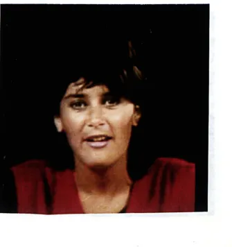
The three algorithms were implemented and tested on three images. These were frames taken from the videoconferencing test sequences mentioned earlier. The sequences are called "Miss America", "Split Screen" and "Trevor White".

Figures 2.14, 2.15 and 2.16 portray the test images. It is apparent that these images vary considerably in their content and complexity. "Miss America" contains by far the least complexity in luminance variation, but the face, with its many subtle changes in flesh tones, occupies a large part of the image, and the pink of the model's sweater is fairly saturated. The backing curtain in the "Split Screen" image seems fairly equiluminou~ but in fact contains a considerable

variation in intensity. The majority of colours in this image are unsaturated, however. The "Trevor White" image is by far the most complex; the texture in

the curtain and in the shirt is difficult to quantise without distortion. Note also the saturated colours in the red polka-dot handkerchief in the model's pocket.

The experimental conditions under which all images were viewed are described in appendix A. The details of these conditions will be discussed further

(66)

Figure 2.14. Original digitised frame from the video

codec test sequence "Miss America". The

image resolution is 256x256 pixels.

(67)

Figure 2.15. Original digitised frame from the video

codec test sequence "Split Screen". The

image resolution is 256x256 pixels.