Optimization of Geometry at Hartree Fock level Using the Generalized Simulated Annealing

Optimization of Geometry at Hartree-Fock Level Using the

Generalized Simulated Annealing

Luiz Augusto Carvalho Malbouisson1, Antonio Moreira de Cerqueira Sobrinho1,

Marco Antônio Chear Nascimento2_{, Miceal Dias de Andrade}1*

1_{Instituto de Física, Universidade Federal da Bahia, Salvador, Brazil} 2_{Instituto de Química, Universidade Federal do Rio de Janeiro, Rio de Janeiro, Brazil}

Email: *_{[email protected]}

Received July 11, 2012; revised August 11, 2012; accepted August 17, 2012

ABSTRACT

This work presents a procedure to optimize the molecular geometry at the Hartree-Fock level, based on a global opti-mization method—the Generalized Simulated Annealing. The main characteristic of this methodology is that, at least in principle, it enables the mapping of the energy hypersurface as to guarantee the achievement of the absolute minimum. This method does not use expansions of the energy, nor of its derivates, in terms of the conformation variables. Dis-tinctly, it performs a direct optimization of the total Hartree-Fock energy through a stochastic strategy. The algorithm was tested by determining the Hartree-Fock ground state and optimum geometries of the H2, LiH, BH, Li2, CH+, OH−,

FH, CO, CH, NH, OH and O2 systems. The convergence of our algorithm is totally independent of the initial point and do not require any previous specification of the orbital occupancies.

Keywords: Geometry Optimization; Hartree-Fock Absolute Minimum; Generalized Simulated Annealing

1. Introduction

The global optimization problem is a subject of intense current interest. Stochastic optimization methods have been utilized to solve this kind of problem. Essentially these methods consist of performing a direct optimization of a given function, denominated cost function, E, within

a determinated stochastic strategy. The Monte Carlo method (MC) is a well-known example of this kind of

method. It has been proposed by Metropolis and Ulam [1] whose presented it as a general purpose tool1_{. In the} sto-chastic strategy applied by Metropolis and Ulam, it is used a function, g, to calculate the visiting probability of

the hypersurface definited by the cost function, _eE k TB 2.

In the original concept of the MC method, the system

configurations randomly chosen and used in the calcula-tions of E, are supposed equiprobable. Metropolis [2]

proposed a modification in the MC algorithm, i.e. he

gave distinct weights to distinct configurations. This method is known in the literature concerned as the Me-tropolis method. Kirkpatrick et al. [3,4] proposed a new

procedure denominated the Simulated Annealing (SA)

method, which is a modification of the Metropolis method [2]. In the SA method, g is a gaussian function

and the T parameter is no longer considered a constant

and changes according to T t

 

T0 log 1



t



, where t

enumerates the cycles of the process. In the literature this method is referred to as the Classical Simulated Anneal-ing (CSA) method or Boltzmann Machine. Szu and

Hart-ley [5] proposed a modification in the CSA method where

the g function is a Cauchy-Lorentz function and T varies

according to T t

 

T0



1t



. The Szu and Hartley

procedure became known in the literature as the Fast Simulated Annealing (FSA) method or Cauchy Machine.

These SA methods have been applied in distinct

situa-tions such as restoration of degraded images [6] and mi-croprocessor circuitry design [4].

The Generalized Simulated Annealing method (GSA)

[7], has been developed and includes both procedures, the FSA and CSA, as special cases. The GSA approach

uses the Tsallis statistics [8,9] to define the visiting dis-tribution function g and has been applied successfully in

the description of a variety of global extremization prob-lems. In the domain of the atomic and molecular aggre-gates, for example, the discovery of the lowest-energy conformations for biological macromolecules or crystal structures for systems with known composition is a fre-quent goal. In particular, the GSA approach has been

used with success in the prediction of new three-dimen- *_{Corresponding author.}

1_{According to a citation in the article by Metropolis [2], this method} was also proposed independently by J. E. Mayer in the study of liquids. 2

kB it is the Boltzmann constant; T is a noise control parameter, usually

sional protein structure and protein folding [10,11], fit-ting the potential energy surface for path reaction and chemical reaction dynamics [12,13], gravimetric problem [14], mechanical properties in alloys [15-17], in elec-tronic structure problems [18-20], among others.

It is important to point out that those typical method-ologies used to treat optimization problems based on solving nonlinear necessary-condition equations do not guarantee the achievement of the absolute minimum. This is the case with some variational electronic structure methods, for instance, the Hartree-Fock (HF), multi-

configuration selfconsistent field (MCSCF), molecular

geometry determination problems and the correspondent methods in the scope of the Nuclear-Electronic Orbital theory (NEO) [21-26]. Moreover, it should be observed

that the absolute minimum of the functional energy in a given class of functions is the best description of the ground state, as the energy is concerned, within that given class. These observations suggest the importance of developing direct optimization methods for studying these classes of extremal problems.

In previous works [18,19], the GSA algorithm was

used to study the problem of determining the absolute minimum of the restricted Hartree-Fock-Roothaan (RHF)

[27] and of the unrestricted Hartree-Fock-Pople-Nesbet (UHF) [28] functionals. In another work the GSA

algo-rithm was applied to construct atomic bases [20]. The method presented in this work is also based on the GSA

algorithm, and it is used to determine the absolute mini-mum and optimini-mum geometry at the Hartree-Fock (HF)

level. This geometry optimization method (hereafter re-ferred to as HFg, RHFg or UHFg) was tested by

deter-mining the HF ground state and optimum geometries of

the H2, LiH, BH, Li2, CH+, OH−, FH, CO, CH, NH, OH and O2 molecules, using minimal, double-zeta and dou-ble-zeta with polarization basis functions (d functions for Li, B, F and p functions for H). The main characteristic

of this methodology is that it enables the mapping of the potential energy hypersurface in order to guarantee, at least in principle, that the absolute minimum of the func-tional in focus is achieved. This methodology does not use expansions of the energy, or of its derivatives, in terms of the conformation variables [29,30]. Distinctly, a direct optimization is performed of the total Hartree-Fock energy function through a stochastic strategy, the GSA

method. A detailed discussion about the multiple HF

extrema, the HF absolute minimum and the GSA

algo-rithm can be found in [18,31-37].

2. The Real

HF

g

Functional and the

Constraint Equations

Since the Roothaan and Pople-Nesbet problems are very well known and documented in the literature, only the more general UHFg functional and constraint conditions

will be presented. Consider a molecular system with

nu-clear coordinates X

 

R_ , n electrons, m atomic basis

functions ξ



 1, , ,2  m



and nnn occupied

LCAO3 molecular orbitals (MOs)





1, 2, , , 1, 2, , ,

; 1, , ; , ,

n n

i i i n

 

       

 



     

   

  _{ } _

 

  

ξ ξ ξc

  



;



where i



c is a column vector with componentsc1i, ,cmi

 _  _, 

 is the matrix m n  formed by the n columns vectors 1, , ,2 n

  _c

c c  . _{ } , _ is the matrix



n



m n_ _ formed by the n_n_ columns vectors 1, , ,2 n_, 1, 2, , n_

  _{ c} _c _c _{ c}

c c . The number m of atomic

functions must satisfy the condition mn_ and mn . The electronic energy functional (in atomic units), in the real UHF approximation, is given by,





ele

1 2

1 2

,

n m

i i

i

n m

j j

j

n m

j j

j

E

c c

h c c

c c







     

 

        

 

     

  

     

   





 _ 

 

 

 _ 

 

 



 

  

X



with the constraint conditions given by,

0 ; 1, , ; , .

m

i j ij

c c _{   } i j n_



        



 (1)

In the above equations    ,  h and    

    are the usual overlap, kinetic energy plus nuclear attraction, and electronic repulsion integrals, re-spectively, that depend of the nuclear coordinates

 





X R . For the HFg functional, the total energy E, is

given by,



,



ele



,



Z Z

E E  

  _{ }

 





X X

R R

  .



(2)

3. The

HF

g

Algorithm

As in references [18-20], the GSA algorithm used here

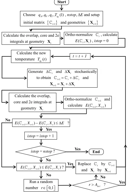
includes two additional modifications relative to the original version described in reference [7]. The first one is the introduction of constraint conditions in the struc-ture of the algorithm (steps 4) and 9)) to treat our varia-tional problem of constrained extrema. The second modi-fication was the introduction of a new independent pa-rameter, _T, to construct the temperature function de-fined in the step 6).

q

The procedure used to search for the global and local minima or to map the cost function hypersurface consists in comparing the total energy for two con-secutive values of the and X obtained with the GSA



,

E  X



routine. and X, for two consecutive GSA steps, are

related to the previous ones via random perturbations on the LCAO-MOs coefficients and on the molecular

con-formation, respectively. In each cycle, and X are simultaneous and independently generated.





In summary, the whole UHFg algorithm for mapping

and searching for the global minimum of the total energy surface is:

1) Fix the qA, qV and qT parameters relative to

accep-tance and visitation probability-distribution functions and temperature function, respectively;

2) Start at t = 1, the first step in the iterative process,

with an arbitrary initial matrix guess t, an arbitrary

molecular conformation and a high enough value for the “temperature” ;



t

X

 

t

T

q

3) Calculate the integrals

T

t

 

  , _ h_{ t} and

t

   

    at Xt;

4) Ortho-normalize the n_ LCAO-MOs vectors

1, 2, ,

t t tn_

 

c c  c



according to Equations 1;

5) Calculate the total energy using

Equa-tion 2;



,

t Xt



E

6) Calculate a new temperature as follows [7]:

 

 





1 1 2 1 1 ; 1 1 T

T T T

q

q q q

T t T

t      

7) Generate randomly the increments



1 1

t g 





  and 1



2

t g 





X 

 

2 2 t

  X

, where

and , are randomly gener-ated by using the visiting probability distribution q_V

 

1 1 t

  

g [7]

to obtain the new matrix t and the new

molecular conformation t1 t

      t 1

t  t 

X X X ;

8) Calculate the integrals ₁

t

 

  _ , _ h_{ t1}

and

1

t

    _ t1

9) Ortho-normalize the new LCAO-MOs vectors

    at X ;

 t 1 1,  t 1 2, ,  t 1n

  

  

c c  c according to Equations 1;

10) Calculate the total energy using Equation 2. The new energy value will be accepted or not according to the rule:



t 1, t 1



E _ X_

if E



t1,Xt1



E



t,Xt



, replace tby t1 and by ,

t Xt1



,





E X E

X

if t1 t1 t,Xt



run a random number

 

0,1 rAacc

r , if , the acceptance probability [7]

de-fined by











 







acc 1 1 1

1, 1 ,

1 1 1 A

T

q t t t t A q A E E q T t                          X X   ,

retain t and , otherwise, replace and by

and ;

 X_t

1

t t

t

 X_t

1

t

11) Take and return to 6) until the conver-gence of

 X_t1



t1,Xt 1



E  is reached within the desired

criterion.

After convergence is achieved, the orbital energies 1, , n_ , ,

 

      are obtained calculating

 

,

i i i

    _,

 c F  c    , where F

 



,

n m

 

is the Fock’s matrix constructed with the converged UHFg

oc-cupied matrix . Also, it is always possible to obtain the virtual canonical vectors,  1



, ,   , 

c  c

, ,

n m

 and the respective virtual orbital energies _1 by diagonalization of the pseudo-eigenvalue equations

 

    _{, ,}

i i i   

c c



F S  [28]. Note that, while for the standard RHF/UHF-SCF [27,28] calculations one

needs to specify, a priory, the orbital occupancy, no ad hoc orbital occupation rule is needed for the RHFg and

UHFg calculations

The following stopping criterion was adopted for the

HFg iterative process convergence was assumed if the

difference between the current total energy value and the lowest total energy previously obtained during the proc-ess was lproc-ess than a pre-established value



E



for a

certain number of consecutive steps (nstop). The HFg

calculations were performed in atomic units and was

used and . The

algo-rithm HFg described above is illustrated in the flowchart

of Figure 1.

11

10

E  hartre

  es nstop10

Start

1 1

( t , t ) ( ,t t)

E X E X  E ?

istop = nstop ?

1 1

( t , t ) ( ,t t)

E X E X ?

End

Ortho-normalize t, calculate

( t, t)

E X , istop = 0

Calculate the new temperature ( )

T

q

T t

Calculate the overlap, core and 2e integrals at

geometry Xt

Ortho-normalize t1 and

calculate E(t1,Xt1)

istop = istop + 1

Yes Yes Yes

Choose q q q TA, V, ,T qT(1), nstop, ΔE and setup initial matrix  t1 and geometries  Xt1

No

t = t + 1

Yes

No _No

Replace t by t1

and Xt by Xt1

Calculate the overlap, core and 2e integrals at geometry Xt

Generate t and Xt stochastically

to obtain t1t t and

1

t  t  t

X X X

No

Run a random

[image:3.595.311.532.385.724.2]

number r  _0,1_ rAacc ?

4. Discussion

To test the HFg method, we calculated the HF ground

state energy and optimum geometry for the H2, LiH, BH,

Li2, CH+, OH–, FH, CO, CH, NH, OH and O2 molecules. The calculations were carried out using minimal (STO-

6G), double-zeta, and double-zeta with polarization

func-tions (d functions for Li, B, F and p functions for H)

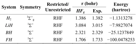
[image:4.595.56.286.273.451.2]

ba-sis sets. Tables 1-3 show the point and spin symmetry classes of the ground state, the kind of calculations per-formed, the geometry and correspondent energy obtained and the experimental geometry extracted from the Herz-berg book [38].

Table 1. Converged HFg energies and geometries using

STO-6G basis.

r (bohr) System Symmetry _UnrestrictedRestricted/

HFg Exp.

Energy (hartree)

[image:4.595.59.286.490.624.2]

H2 1+g RHF 1.343 1.382 −1.126216 LiH 1+ RHF 2.847 3.015 −7.953471 BH 1+ RHF 2.276 2.329 −25.001901 Li2 1+g RHF 5.082 5.051 −14.808883 CH+ 1_+ _{RHF 2.237 2.137 −37.827055} OH– 1_+ _{RHF 2.015 1.833 −74.786010} FH 1+ RHF 1.803 1.733 −99.501719 CO 1+ RHF 2.165 2.132 −112.304213 CH 2 UHF 2.151 2.116 −38.145699 NH 3– UHF 2.038 1.958 −54.794662 OH 2 UHF 1.912 1.832 −75.078694 O2 3–g UHF 2.301 2.282 −149.052202 Table 2. Converged HFg energies and geometries using DZ

basis.

r (bohr) System Symmetry _UnrestrictedRestricted/

HFg Exp.

Energy (hartree)

[image:4.595.309.540.539.719.2]

H2 1+g RHF 1.379 1.382 −1.1267990 LiH 1+ RHF 3.104 3.015 −7.9810243 BH 1+ RHF 2.345 2.329 −25.1134219 CH+ 1_+ _{RHF 2.108 2.137 −37.8850797} OH– 1+ RHF 1.845 1.833 −75.3509506 FH 1+ RHF 1.738 1.733 −100.0219016 CO 1+ RHF 2.150 2.132 −112.6850704 CH 2+ UHF 2.111 2.116 −38.2589640 NH 3– UHF 1.959 1.958 −54.9549663 OH 2+ UHF 1.833 1.832 −75.3860061 Table 3. Converged HFg energies and geometries using DZ

polarized basis.

r (bohr) System Symmetry _UnrestrictedRestricted/

HFg Exp.

Energy (hartree)

H2 1+g RHF 1.386 1.382 −1.1313278 LiH 1+ RHF 3.084 3.015 −7.9827074 BH 1+ RHF 2.321 2.329 −25.1237849 FH 1+ RHF 1.706 1.733 −100.0478253

We performed several RHFg and UHFg calculations

combining different initial values with distinct sets of the parameters qA, qV, qT and T0. We found that the narrow ranges of values of the parameters qV and qT,

leading to a better convergence (smallest number of HFg

cycles), namely,



,X





2.6, 2.9





V

q and q_T



1.6, 2.0



, e

similar to those obtained in previous works [18,19]. In particular, for the minimal basis set, the best convergence is achieved for qV 2.9

 ar

 and qT 1.9, which are quite

close to the best values obtained for the RHF-GSA and UHF-GSA problems [18,19]. In addition, we performed

several calculations using different values of qA,

includ-ing Aacc0, wh the convergence, therefore, been adopted in step 10) of the HFg algorithm, an

accep-tance probability, _acc ich led to

A , equal zero for all calculations.

The genera

to onvergence be

l g

algo-rit

c havior of the HF

hm is similar to that of the RHF-GSA and UHF-GSA

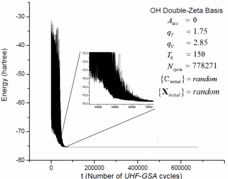
methods [18,19]. For all systems and bases sets em-ployed, it was always possible to obtain the global mini-mum, with several distinct combinations of these pa-rameters, each set of parameters requiring a different number of HFg cycles. Also in all calculations, the HFg

energies initially show a strong oscillatory behavior but soon afterwards the energy starts to smoothly converge towards the absolute minimum. Figures 2 and 3 present the RHFg and UHFg convergence profiles for the CH+

and OH molecules, indicating the values of the

parame-ters Aacc, qV, qT, T0, the atomic basis sets, the type of guess for the initial values of 



_initial



and X



Xinitial



, and the number of the cy le ich

was achieved

c s for wh

vergence



N_cycle



. Similar convergence

profiles were obtained for thers molecules. In order to verify the accuracy of the calculation

all the o

s, the

RHFg and UHFg results were compared with those

ob-tained by the standard gradient RHF/UHF geometry

cal-culation method, for all molecules considered, using the

[image:4.595.58.287.663.737.2]

[image:5.595.58.286.85.264.2]

Figure 3. OHdouble-zeta basis HFgconvergence process.

program GAMESS [39]. Three choices for the initial

ma--G

-tio

F

-ure GSA used in the pre

w

financial support: FAPERJ

[1] A N. Metrop The Monte Carlo

trix  were considered when performing the RHF/ UHF AMESS calculations: the eigenvectors of core

hamiltonian (Hcore₎4_{, the eigenvectors of an extended} Huckel calculations (Huckel)5_{, and the eigenvectors of a} previous RHFg or UHFg calculation. Furthermore,

when-ever necessary, the Direct Inversion in the Iterative Sub-space (DIIS) convergence acceleration technique [40,41]

was also used for the RHF/UHF-GAMESS calculations.

In all cases we examined, the RHFg and UHFg calcula

ns converge to the global minimum with any randomly generated initial  and X values, what is not observed for the RHF/UH GAMESS calculations. Besides, the HFg method do not need any previous specification of

the orbital occupancies.

The stochastic proced vious orks [18-20] and in this paper can be extended to other variational approaches, for instance, the Multi-Configu-ration Self-Consistent method [42] and in the Nuclear- Electronic Orbital theory [21-26]. Works in this direction are in progress.

5. Acknowledgements

M. A. C. Nascimento thanks

(of Brazil); CAPES (of Brazil) and CNPq (of Brazil).

REFERENCES

olis and S. Ulam, “

Method,” Journal of the American Statistical Association,

Vol. 44, No. 247, 1949, pp. 335-341. doi:10.1080/01621459.1949.10483310

. Rosenbluth, A. [2] N. Metropolis, A. W. Rosenbluth, M. N

H. Teller and E. Teller, “Equation of State Calculations by Fast Computing Machines,” Journal of Chemical

Physics, Vol. 21, No. 6, 1953, pp. 1087-1092.

doi:10.1063/1.1699114

[3] S. Kirkpatrick, C. D. Gelatt Jr. and M. P. Vecchi, “Opti-mization by Simulated Annealing,” Science, Vol. 220, No.

8, 1983, pp. 671-680. doi:10.1126/science.220.4598.671 [4] S. Kirkpatrick, “Optimization by Simulated Annealing:

Quantitative Studies,” Journal of Statistical Physics, Vol.

34, No. 5-6, 1984, pp. 975-986. doi:10.1007/BF01009452 [5] H. Szu and R. Hartley, “Fast Simulated Annealing,”

Physics Letters A, Vol. 122, No. 3-4, 1987, pp. 157-162.

doi:10.1016/0375-9601(87)90796-1

[6] S. Geman and D. Geman, “Stochastic Relaxation, Gibbs Distributions, and the Bayesian Restoration of Images,”

IEEE Transactions on Pattern Analysis Machine Intelli- gence, Vol. 6, 1984, pp. 721-741.

doi:10.1109/TPAMI.1984.4767596

eneralized Simulated [7] C. Tsallis and D. A. Stariolo, “G

Annealing,” Physica A, Vol. 233, No. 1-2, 1996, pp. 395-

406. doi:10.1016/S0378-4371(96)00271-3

[8] C. Tsallis, “Possible Generalization of Boltzmann-Gibbs Statistics,” Journal of Statistical Physics, Vol. 52, 1988,

pp. 479-487. doi:10.1007/BF01016429

[9] E. M. F. Curado and C. Tsallis, “Generalized Statistical Mechanics: Connection with Thermodynamics,” Journal of Physics A: Mathematical and General, Vol. 24, No. 2,

1991, p. L69; Journal of Physics A: Mathematical and General, Vol. 24, No. 4, 1992, p. 1019 (Corrigendum). doi:10.1088/0305-4470/25/4/038

[10] M. A. Moret, P. G. Pascutti, P. M. Bisch and K. C.

Mun-47::AID dim, “Stochastic Molecular Optimization Using General-ized Simulated Annealing,” Journal of Computational Chemistry, Vol. 19, No. 6, 1998, pp. 647-657.

doi:10.1002/(SICI)1096-987X(19980430)19:6<6 -JCC6>3.0.CO;2-R

[11] M. A. Moret, P. M. Bisch, K. C. Mundim and P. G. Pascutti, “New Stochastic Strategy to Analyze Helix Folding,” Biophysical Journal, Vol. 82, No. 3, 2002, pp.

1123-1132. doi:10.1016/S0006-3495(02)75471-4

[12] L. E. Espinola, R. Gargano, K. C. Mundim and J. J. Soares Neto, “The Na+ _{HF Reactive Probabilities} Calcu-lations Using Two Different Potential Energy Surfaces,”

Chemical Physics Letters, Vol. 361, No. 3-4, 2002, pp. 271-276. doi:10.1016/S0009-2614(02)00924-7

[13] A. F. A. Vilela, J. J. Soares Neto, K. C. Mundim, M. S. P. Mundim and R. Gargano, “Fitting Potential Energy Sur-face for Reactive Scattering Dynamics through General-ized Simulated Annealing,” Chemical Physics Letters,

Vol. 359, No. 5-6, 2002, pp. 420-427. doi:10.1016/S0009-2614(02)00597-3

[14] K. C. Mundim, T. J. Lemaire and A. Bassrei, “Optimiza-tion of Non-Linear Gravity Models through Generalized Simulated Annealing,” Physica A, Vol. 252, No. 3-4,

1998, pp. 405-416. doi:10.1016/S0378-4371(97)00634-1 [15] K. C. Mundim and D. E. Ellis, “Stochastic Classical

Mo-lecular Dynamics Coupled to Functional Density Theory: Applications to Large Molecular Systems,” Brazilian Journal of Physics, Vol. 29, No. 1, 1999, pp. 199-214. doi:10.1590/S0103-97331999000100018

orfman a

son, K. C. Mun-[16] D. E. Ellis, K. C. Mundim, D. Fuks, S. D nd A.

Berner, “Interstitial Carbon in Copper: Electronic and Mechanical Properties,” Philosophical Magazine Part B,

Vol. 79, No. 10, 1999, pp. 1615-1630. [17] S. Dorfman, D. Fuks, L. A. C. Malbouis

dim and D. E. Ellis, “Influence of Many-Body Interac-tions on Resistance of a Grain Boundary with Respect to a Sliding Shift,” International Journal of Quantum Chemistry, Vol. 90, No. 4-5, 2002, pp. 1448-1456. doi:10.1002/qua.10357

[18] M. D. de Andrade, K. C. Mundim and L. A. C. Mal- bouisson, “GSA Algorithm Applied to Electronic Struc- ture: Hartree-Fock-GSA Method,” International Journal of Quantum Chemistry, Vol. 103, No. 5, 2005, pp. 493- 499. doi:10.1002/qua.20580

[19] M. D. de Andrade, K. C. Mundim, M. A. C. Nascimento and L. A. C. Malbouisson, “GSA Algorithm Applied to Electronic Structure II: UHF-GSA Method,” Interna-tional Journal of Quantum Chemistry, Vol. 106, No. 13, 2006, pp. 2700-2705. doi:10.1002/qua.21080

[20] M. D. de Andrade, M. A. C. Nascimento, K. C. Mundim, A. M. C. SOBRINHO and L. A. C. Malbouisson, “Atomic Basis Sets Optimization Using the Generalized Simulated Annealing Approach: New Basis Sets for the First Row Elements,” International Journal of Quantum Chemistry, Vol. 108, No. 13, 2008, pp. 2486-2498.

doi:10.1002/qua.21666

[21] S. P. Webb, T. Iordanov and S. Hammes-Shiffer,

“Multi- s-configurational Nuclearelectronic Orbital Approach: In- corporation of Nuclear Quantum Effects in Electronic Structure Calculations,” International Journal of Quan- tum Chemistry, Vol. 117, No. 9, 2002, pp. 4106-4118.

[22] M. V. Pak, C. Swalina, S. P. Webb and S. Hamme Shiffer, “Application of the Nuclear-Electronic Orbital Method to Hydrogen Transfer Systems: Multiple Centers and Multiconfigurational Wavefunctions,” Chemical Physics, Vol. 304, No. 1-2, 2004, pp. 227-236.

doi:10.1016/j.chemphys.2004.06.009

[23] C. Swalina, M. V. Pak and S. Hammes-Shiffer. “Analysis of the Nuclear-Electronic Orbital Method for Model Hy-drogen Transfer Systems,” Journal of Chemical Physics,

Vol. 123, No. 1, 2005, p. 14303. doi:10.1063/1.1940634 [24] A. Reyes, M. V. Pak and S. Hammes-Shiffer, “Investiga-

tion of Isotope Effects with the Nuclear-Electronic Or- bital Approach,” Journal of Chemical Physics, Vol. 123,

No. 6, 2005, p. 64104. doi:10.1063/1.1990116

[25] J. H. Skone, M. V. Pak and S. Hammes-Shiffer, “Nu- clear-Electronic Orbital Nonorthogonal Configuration In-teraction Approach,” Journal of Chemical Physics, Vol.

123, No. 13, 2005, p. 134108. doi:10.1063/1.2039727 [26] C. Swalina, M. V. Pak, A. Chakraborty and S. Hammes-

Shiffer, “Explicit Dynamical Electron-Proton Correlation in the Nuclear-Electronic Orbital Framework,” Journal of

Chemical Physics A, Vol. 110, No. 33, 2006, pp.

9983-9987. doi:10.1021/jp0634297

[27] C. C. J. Roothaan, “New Developments in Molecular Orbital Theory,” Reviews of Modern Physics, Vol. 23, No.

2, 1951, pp. 69-89. doi:10.1103/RevModPhys.23.69 8] J. A. Pople and R. K. Nesbet, “Self-Consistent Orb

[2 itals

for Radicals,” Journal of Chemical Physics, Vol. 22, No.

3, 1954, pp. 571-572. doi:10.1063/1.1740120

[29] D. B. Cook, “Handbook of Computational Chemistry,”

Chemis-ams, “Stability of Hartree-Fock States,” Physi-

Oxford University Press, Oxford, 1998, p. 671. [30] A. Szabo and N. S. Ostlund, “Modern Quantum

try: Introduction to Advanced Electronic Structure The-ory,” Dover Publications, New York, 1996, Appendix C, pp. 444.

[31] W. H. Ad

cal Review, Vol. 127, No. 5, 1962, pp. 1650-1658.

doi:10.1103/PhysRev.127.1650

[32] R. E. Stanton, “Multiple Solutions to the Hartree-Fock Problem I. General Treatment of Two-Electron Closed- Shell Systems,” Journal of Chemical Physics, Vol. 48,

No. 1, 1968, pp. 258-262. doi:10.1063/1.1667913

[33] J. C. Facelli and R. H. Contreras, “A General Relation between the Intrinsic Convergence Properties of SCF Hartree-Fock Calculations and the Stability Conditions of Their Solutions,” Journal of Chemical Physics, Vol. 79,

No. 7, 1983, pp. 3421-3423. doi:10.1063/1.446190 [34] L. A. C. Malbouisson and J. D. M. Vianna, “An

Alge-ra Filho, L. A. C. Malbouisson and J. D. M. braic Method for Solving Hartree-Fock-Roothaan Equa-tions,” Journal of Chemical Physics, Vol. 87, 1990, pp.

2017-2025. [35] R. M. Teixei

Vianna, “An Algebraic Method for Solving Hartree-Fock Equations II. Open-Shell Molecular Systems,” Journal of Chemical Physics, Vol. 90, No. 10, 1993, pp. 1999-2005.

[36] L. E. Dardenne, N. Makiuchi, L. A. C. Malbouisson and J. D. M. Vianna, “Multiplicity, Instability, and SCF Con-vergence Problems in Hartree-Fock Solutions,” Journal of Quantum Chemistry, Vol. 76, No. 5, 2000, pp. 600-610.

doi:10.1002/(SICI)1097-461X(2000)76:5<600::AID-QU A2>3.0.CO;2-3

[37] K. N. Kudin, G. E. Scuseria and E. Cancès, “A Black-Box Self-Consistent Field Convergence Algorithm: One Step Closer,” Journal of Chemical Physics, Vol. 116,

No. 19, 2002, pp. 8255-8261. doi:10.1063/1.1470195 [38] K. P. Huber and G. Herzberg, “Constants of Diatomic

. T. Elbert, Molecules,” Van Nostrand, New York, 1979.

[39] M. W. Schmidt, K. K. Baldridge, J. A. Boatz, S

M. S. Gordon, J. H. Jensen, S. Koseki, N. Matsunaga, K. A. Nguyen, S. J. Su, T. L. Windus, M. Dupuis and J. A. Montgomery, “General Atomic and Molecular Electronic Structure System,” Journal of Computational Chemistry,

Vol. 14, No. 11, 1993, pp. 1347-1363. doi:10.1002/jcc.540141112

[40] P. Pulay, “Convergence Acceleration of Iterative Se-quences. The Case of SCF Iteration,” Chemical Physics Letters, Vol. 73, No. 2, 1980, pp. 393-398.

doi:10.1016/0009-2614(80)80396-4

[41] P. Pulay, “Improved SCF Convergence Acceleration,”

Journal of Computational Chemistry, Vol. 3, No. 4, 1982,

pp. 556-560. doi:10.1002/jcc.540030413