An approximate Itô-SDE based simulated annealing algorithm for multivariate design optimization problems

arXiv:1901.10763v1 [math.OC] 30 Jan 2019

An approximate Itˆ

o-SDE based simulated annealing algorithm for

multivariate design optimization problems

A. Batou

Universit´e Paris-Est, Laboratoire Mod´elisation et Simulation Multi Echelle,

MSME UMR 8208 CNRS, France

January 31, 2019

Abstract

This research concerns design optimization problems involving numerous design parameters and large computational models. These problems generally consist in non-convex constrained optimization prob-lems in large and sometimes complex search spaces. The classical simulated annealing algorithm rapidly loses its efficiency in high search space dimension. In this paper a variant of the classical simulated annealing algorithm is constructed by incorporating (1) an Itˆo stochastic differential equation generator (ISDE) for the transition probability and (2) a polyharmonic splines interpolation of the cost function. The control points are selected iteratively during the research of the optimum. The proposed algorithm explores efficiently the design search space to find the global optimum of the cost function as the best control point. The algorithm is illustrated on two applications. The first application consists in a simple function in relatively high dimension. The second is related to a Finite Element model.

Keywords: Engineering Design; Simulated annealing; Itˆo stochastic differential equation; polyhar-monic spline interpolation)

1

Introduction

Recent advances in computational mechanics offer engineers the possibility of constructing very predictive computational models of complex mechanical structures. Such computational models can then be used to assess the performance of the structure over specific design scenarios. This increase of predictability is inevitably accompanied by an increase of the size of the computational models. In most industrial sectors, it is common for engineers to deal with computational models having tens of millions of degrees of freedom. The forward problem consisting in calculating the response of an already designed system can be performed using usual computational resources. Nevertheless the design of a system represented by a large computational model is a hard task since it generally consists in a large non-convex constrained optimization problem in a large and sometimes complex search space and requires numerous runs of the cost function.

Many researches have been devoted to the extension of simulated annealing method to multiobjective opti-mization problems [Suman and Kumar(2006)]. The improvement of the annealing schedule has also interested many researchers (see for instance [Kouvelis and Chiang(1992)] for the choice of the initial temperature and [Ingber(1989), Noutani and Andresen(1998), Azizi and Zolfaghari(2004), Triki, Collette, and Siarry(2004)] for the cooling schedule). Convergence results related to simulated annealing algorithm have been studied in [Aarts and Laarhoven(1985), Lundy and Mees(1986), Faigle and Schrader(1988), Faigle and Kern(1991), Granville, Krivanek, and Rasson(1994)] for the case where the temperature is held constant until a stationary

distribution is reached and in [Mitra, Romeo, and Sangiovanni-Vincentelli(1986), Hajek(1988), Connors and Kumar(1989), Borkar(1992), Anily and Federgruen(1987), Yao and Li(1991)] for the case where the temperature always

changes (and then no stationary distribution can be reached). For cost functions involving large computa-tional models, the simulated annealing algorithm can become prohibitively time consuming. To circumvent this difficulty, an adaptative surface response can be introduced for the approximation of the cost function [Wang, Dong, and Aitchison(2001)].

The basic version of the simulated annealing [Kirkpatrick, Gelatt, and Vecchi(1983), ˇCern´y(1985)] is based on a Metropolis-Hastings algorithm [Hastings (1970)] for which a proposal distribution has to be provided. If the dimension of the search spaces increases, it is not easy to defined this proposal distribution and the Markov chain can become very slow due to numerous rejections. In this case, for large computational models, the use of the classical simulated annealing algorithm can become prohibitive due to the large number of runs of the cost function that are needed.

The objective of this paper is to improve the simulated annealing algorithm in order to design, in high-dimensional search space, complex mechanical systems represented by large computational models. The methodology proposed in the present paper is based on two ingredients. The first one consists in replacing the Metropolis-Hastings algorithm by an Itˆo stochastic differential equation (ISDE) generator [Soize(1994), Soize(2008)] which belongs to class of Monte Carlo Markov Chain Methods (MCMC). This generator is very well adapted in high dimension and does not require the specification of a proposal distri-bution. Nevertheless it requires the gradient of the cost function to be evaluated thousands times making it unusable. To circumvent this difficulty, the second ingredient of the methodology proposed here consists, as in [Wang, Dong, and Aitchison(2001)], in introducing response surface function in order to approximate the cost function. Since we are interested in multivariate optimization problems, a radial interpolation surface (polyharmonic) is preferred to a polynomial approximation (as used in[Wang, Dong, and Aitchison(2001)]). This interpolation is well adapted in relatively high input dimension and allows the gradient of the cost function to be calculated explicitly at each step of the Markov Chain. An adaptative strategy is proposed in order to enrich sequentially, during the numerical integration of the ISDE, the set of the control points that are used to construct the interpolation surface. At the end of the simulation the best control point is selected as the global optimum.

In Section 2, the design optimization problem and the classical simulated annealing algorithm are pre-sented. Then Section 3 is devoted to the presentation the ISDE-based simulated annealing algorithm. The constraints on the design parameters are taken into account by introducing a regularisation of the indicator function. In Section 4, the polyharmonic interpolation of the cost function is introduced and the complete approximate ISDE-based simulated annealing algorithmdesign optimization algorithm is presented. The methodology is illustrated through two applications in Section 5. The first application consists in the classi-cal Ackley’s test function in high dimension. The second one consists in a Finite Element structure submitted to an acceleration of the soil and for which the maximal displacement has to be minimized by designing the stiffnesses of supporting springs.

2

Design optimization problem and classical simulated annealing

algorithm

In this section the design optimization problem is formulated and the simulated annealing probability distri-bution is constructed classically using the Maximum Entropy (MaxEnt) principle.

Leta_{be the vector of the design parameters with values inR}N_{. LetC}

a ⊆RN be the admissible set for

minimum of a non-convex positive cost functionD(a_{). Then the optimal value}aopt _{of vectorais calculated}

such that

aopt_{= arg min}

a∈CaD

(a_{). (1)}

For instance, in case of a least square problem, the function D(a_{) can be written as}

D(a_{) =k}G(a₎₋g∗_k2, (2) in whichG(a_{) is a performance vector-valued function and}g∗is a target vector. In random search methods, a random vector A _{with values in Ca is associated with the vector} a_{. In the simulated annealing the}

probability density function (pdf) pA(a) of random vectorAis constructed by using the MaxEnt principle

[Shannon(1948), Jaynes(1957), Kapur and Kevasan(1992)] under the constraints defined by the available information related to random vectorA_{. This information is written as}

a_{∈ Ca, (a)} Z

Ca

1lCa(a) exp(−λD(a))da) = 1, (b) E{D(a_{)}=c <+∞, (c)}

(3)

in whichE{.}is the mathematical expectation. Equation(3-b) is related to the normalization of the pdf and Eq. (3-c) is related to the finiteness of the mean value of the cost function which is interpreted as an energy in thermodynamics. The entropy related to pdfpA is defined by

S(pA) =−

Z

RN

pA(a) log(pA(a)) da, (4)

where log is the natural logarithm. This functional measures the relative uncertainty of pA. LetC be the

set of all the possible pdfs of random vector A_{, satisfying the constraints defined by Eq. (3). Then the}

MaxEnt principle consists in constructing the pdfpA as the unique pdf inCwhich maximizes entropyS(pA).

Then by introducing a positive Lagrange multiplierλ0associated with Eq. (3-b) and a Lagrange multiplierλ

associated with Eq. (3-c), it can be shown (see [Jaynes(1957), Kapur and Kevasan(1992)]) that the MaxEnt solution, is defined by

pA(a) = 1lCa(a)λ0 exp(−λD(a)) (5)

in which λ0= (R_Ca1lCa(

a_{) exp(−λD(}a_))da₎−1 _{is a normalization constant. In the context of the simulated}

annealing algorithm, the Lagrange multiplier is written asλ= 1

T (orλ=

1

βT withβ >0) in whichT is the

temperature which controls the sharpness of pdfpA. Then random variableAis rewrittenAT and its pdf is

rewritten as

pAT(a) = 1lCa(a)λ0exp(−

D(a₎

T ) (6)

A large value of the temperature makes pAT tend to the uniform distribution and a small value of the

temperature makespAT tend to a Dirac distribution centred at the optimal value. Then the classical simulated

annealing algorithm consists in constructing a sequence (A1_,A2_{, . . . ,}Ant

) using the Metropolis-Hastings (MH) algorithms [Hastings (1970)] with the pdfpAT while decreasing slowly the temperature (see for instance

[Noutani and Andresen(1998)] for the cooling strategies). The algorithm is summarized in Algorithm 1. In this algorithm 1, it is often set Mk = 1 for k = 1. . . , nt, skipping the burning phase. In this case, there

is only one loop and the temperature is changed at each iteration. Under some conditions related to the rate of decreasing of the temperature, the algorithm converges to the global optimum. Two difficulties are usually referred for the classical simulated annealing algorithm:(1) it requires numerous calculation of the cost function D(a_{) making it unusable for large computational model and (2) if the dimension of random design}

vectorA_{T is large, the Metropolis-Hastings algorithms may have difficulties to explore efficiently the design}

search space. In the next sections two modifications are introduced to circumvent these two difficulties. The first one consists in replacing the Metropolis-Hastings generator by an ISDE generator in order to explore efficiently the design search space in high dimension. The second one consists in introducing a polyharmonic spline interpolation of the function a _{7→ D(}a_{) for which the list of control points is enriched during the}

Algorithm 1Classical simulated annealing algorithm

INITIALIZATION:

Generate initial valueA₀ A1₌A₀ LOOP: fork= 1, . . . ,(nt−1) do

Set temperatureTk

Set the sizeMk of the MH sequence

MH algorithm:

forℓ= 1, . . . ,(Mk−1)do

Generate a neighbour Ak,new _ofAk

if _D(Ak,new_)<D(Ak₎then

Ak _←Ak,new

end else

Generateuuniformly in [0,1]

if u <exp(−(D(Ak,new_{)− D(}Ak_))/Tk)then

Ak _←Ak,new

end end end

Ak+1_←Ak

end

3

Construction of a new ISDE-based simulated annealing

algo-rithm

The ISDE generator consists in constructing the pdf of random vector A_{T as the density of the invariant}

measure pAT(a)daassociated with the stationary solution of a second-order nonlinear ISDE. This

method-ology, which has similarities with the Hamiltonian (or Hybrid) Monte Carlo method [Duane, et al(1987), Salazar and Toral(1997)], has recently been revisited [Soize(1994), Soize(2008)] in the context of the genera-tion of random vectors in high dimension for which the pdf is constructed using the MaxEnt principle with complex available information. The advantages of this generator compared to the other MCMC generators such as the Metropolis-Hastings algorithm (see [Hastings (1970)]) are: (1) there is no need to introduce a proposal distribution (uniform in case of random walk) for the exploration of the admissible space, (2) a damping can be introduced in order to rapidly reach the invariant measure and (3) mathematical results concerning ISDEs can be used for convergence analyses. Below, we first present the ISDE generator followed by its application for generating independent realizations ofA_{T. Then a new simulated algorithm based on}

the use of this ISDE generator is presented

3.1

ISDE generator

Let Ψ(u_{) be a positive function. Let{(}U_(r),V_{(r)), r ≥0} be a stochastic process with values inR}N _×RN

satisfying, for all r≥0, the following ISDE [Itˆo(1951), Soize(1994)]

dU_{(r) =} V_{(r) dr}

dV_{(r) = −}∇uΨ(U) dr−1₂[D]V(r) dr+ [S] dW(r),

(7)

with the initial conditions

U_{(0) =}U_{0 ,} V_{(0) =}V_{0 a.s . (8)}

In Eq. (7),∇uΨ(u) is the gradient of function Ψ(u) with respect tou. The matrix [D] is a symmetric

positive-definite damping matrix, the lower triangular matrix [S] is such that [D] = [S][S]T _{andW = (W}

is the normalized Wiener stochastic process indexed by R+. The random initial condition (U_0,V_{0) is a}

second-order random variable independent of the Wiener stochastic process {W_{(r), r ≥0}. Then it can be}

proven (see [Soize(1994), Soize(2008)]) that, if u_7→Ψ(u_{) is continuous onR}N_{, ifu7→ k∇}

uΨ(u)k is locally

bounded onRN (i.e. is bounded on all compact set inRN), and if

inf

kuk>RΨ(

u_{)→+∞ ifR→+∞, (9)}

inf

u∈RNΨ(

u_{) = Φmin with Φmin∈R, (10)}

Z

RNk

∇uΨ(u)kexp(−Ψ(u)) du < +∞, (11)

then the ISDE defined by Eqs. (7) and (8) admits an invariant measure defined by the pdfρ(u_,v_{) which is}

written as

ρ(u_,v_{) =λ0exp(−}∇uΨ(u)×(2π)−N/2exp(−

1 2kvk

2_{). (12)}

It can then be deduced that, for r → +∞, the stochastic process {U_{(r), r ≥ 0} tends to a stationary}

stochastic process in probability distribution, for which the one-order marginal probability distribution is

pUst(u) such that

pUst(u) =λ₀ exp(−Ψ(u)). (13)

Therefore, using an independent realization of the Wiener stochastic process W _{and an independent}

re-alization of the initial condition (U_0,V_{0), an independent realization random variable} Ust _{related to the}

probability distribution (13) can be constructed as the solution of the ISDE defined by Eqs. (7) and (8), for

r sufficiently large. In other words, independent realizations of any random variable having a probability distribution of the form (13) (verifying the required continuity and regularity properties for function Ψ) can be obtained by solving the ISDE defined by Eqs. (7) and (8). The value r0 of r for which the invariant

measure is approximatively reached depends on the choice of the damping matrix [D] and on the probability distribution of the random initial conditions. The damping induced by the matrix [D] has to be sufficiently large in order to rapidly kill the transient response but a too large damping introduces increasing errors in the numerical integration of the ISDE.

The solution of the ISDE can be constructed numerically using a for instance a modified Euler inte-gration schemes which has a better accuracy than a classical Euler inteinte-gration schemes (see [Soize(2008), Burrage(2007)]). Let ∆r be the integration step size and let{rℓ, ℓ= 1, . . . , M} be the sampling points, M

being a positive integer. Let {Uℓ_{, ℓ = 1, . . . , M} and {V}ℓ_{, ℓ = 1, . . . , M} be the time series related to the}

discretization of random processes U_{(r) and}V_{(r). Then, after having generated the random initial values}

U1_=U

0 andV1=V0, the following updating rules applies

Vℓ+1 _{= ([I]−}∆r

2 [D])V

ℓ

−∆r∇uΨ(Uℓ) + [S]∆Wℓ+1,

Uℓ+1 ₌ Uℓ_{+ ∆r}Vℓ+1

(14)

The vector ∆Wℓ+1 _{is a second-order Gaussian centered random vector with covariance matrix equal to}

∆r[IN] and the random vectors ∆W1, . . . ,∆WM are mutually independent.

3.2

ISDE generator for random variable

A

Equation (6) can be rewritten as

pAT(a) = λ0 exp(log(1lCa(a))−

D(a₎

Comparing equations (13) and (15), we naturally introduce the function

ΨT(a) =D

(a₎

T −log(1lCa(a)), (16)

Unfortunately, due to the presence of the indicator function a _{7→ 1lCa(}a_{), the function ΨT(}u_{) is not}

dif-ferentiable and then cannot be used within an ISDE generator. To solve this issue, the indicator func-tion a _{7→ 1lCa(}a_{) is replaced by the regularized indicator function} a _{7→ 1l}reg

Ca(a). For simple manifolds,

explicit regularized indicator function can be constructed. Two simple examples are given below (see [Batou and Soize(2014)]):

Example 1: Positive design variables

Assume that the constraints on a_are

ai>0, i= 1. . . , N . (17)

In this case, the regularized indicator function can be constructed as follow

1lregCa(a) = N

Y

i=1

1 2

1 + tanh

_a

i

αi

, (18)

where αi>0, i= 1. . . , N are shape parameters

Example 2: Design variables belonging to independent intervals

Assume that the constraints on a_are

li< ai< ui, i= 1. . . , N , (19)

whereliandui,i= 1. . . , N are lower and upper bounds. In this case, the regularized indicator function can

be constructed as follow

1lreg_Ca(

a_{) =}

N

Y

i=1

1 4

1 + tanh

ai−li

αi

1 + tanh

ui−ai

αi

. (20)

For more complex manifolds, a general kernel-smoothing regularization approach has been proposed in [Guilleminot and Soize(2014)].

Then a regularized ISDE can be introduced by replacing, in Eq.(7), Ψ by Ψreg_T such that

Ψreg_T (a_{) =}D(a)

T −log(1l

reg

Ca(a)), (21)

and then independent realizations of random variableA_{T can be constructed.}

3.3

ISDE based simulated annealing algorithm

Now that an ISDE generator for random variableA_{T is constructed, we can use this generator for replacing}

the MH algorithm in the classical simulated annealing algorithm 1. This ISDE based simulated annealing algorithm is summarized in Algorithm 2.

At each changing of the temperature, three parameters have to be set: the steps in the ISDE ∆rk, the

damp-ing matrix [Dk] = [Sk][Sk]T and the number of stepsMk in the ISDE. By analogy to second-order dynamical

systems, the time step that guaranties the stability of the modified Euler scheme is calculated using the eigen-values related the conservative part of the dynamical equation. In the ISDE (7), the corresponding ”mass” matrix is identity and the ”stiffness” matrix for given ”displacement” U _{is the hessian matrix [HΨT(}U_{)] of}

function ΨT(U). Then at each iterationk, the step is calculated as ∆rk= 2π/(m√λmax) wheremis an

inte-ger such thatm >10 andλmaxis the largest eigenvalue of the hessian matrix [HΨT(U

1_{)]. When approaching}

the border of the admissible domainCa, the ISDE can become very ”stiff”, which may yield stability issues.

Algorithm 2ISDE-based simulated annealing algorithm

INITIALIZATION:

GenerateU_{0 and}V₀ A1₌U₀

U1₌U₀ V1₌V₀

LOOP:

fork= 1, . . . ,(nt−1) do

Set temperatureTk

Set damping matrix [Dk] = [Sk][Sk]T

Set increment ∆rk

Set number of stepsMk

Solve ISDE :

forℓ= 1, . . . ,(Mk−1)do

Vℓ+1_{= ([I]−}∆rk

2 [Dk])V

ℓ

−∆rk∇uΨreg_Tk(Uℓ) + [Sk]∆Wℓ+1

Uℓ+1₌Uℓ_{+ ∆rk}Vℓ+1

end

Ak+1₌U_Mk U1_←U_Mk V1_←V_Mk

end

the best step-size at each iteration of the Euler Scheme [Guilleminot and Soize(2014)]. The damping matrix has to be large enough in order to kill rapidly the transient response. But a too large damping will introduce errors during the integration. A good compromise consists in imposing the largest damping rate equal to

ξ= 0.7. This can achieved approximatively by choosing [Dk] = 2ξ√λmax[IN]. The number of steps of Mk

can be chosen as invariant and then determined through an off-line convergence analysis. The convergence can also be controlled during the integration of each ISDE yielding different values for M1, . . . , Mk.

4

Approximation of the cost function

In this section, the functiona_{7→ D(}a_{) in the ISDE is approximated using multivariate polyharmonic splines.}

This approximation allows to reduce the computational cost for large computational models. Furthermore it allows to derive explicitly the gradienta_7→∇aD(a), avoiding the calculation of the gradient numerically.

The multivariate polyharmonic splines approximationa_{7→ D}mps_{(a) of function a7→ D(a) is written as} Dmps_{(a) =w}T_{b(a), (22)}

in which b₍a_{) = (b1(}a_{), . . . bnc(}a_{)) is the vector of thenc p-order polyharmonic splines defined atnc control}

pointsc1_{, . . . ,c}nc _{and which are such that, fori= 1, . . . , n} c

bi(a) =ka−cikp ifpis odd,

bi(a) =ka−cikplog(ka−cik) ifpis even.

(23)

For the odd and even cases, ifa₌ci _thenbi(a_{) = 0. In Eq. (22),}w_{is the weight vectors inR}nc_{. Classically,}

this vector should be calculated by solving the set ofnc equations

D(ci_{) =}wTb₍ci_{), i= 1, . . . , nc, (24)}

yielding nc independent equations allowing vectorsw to be calculated. The function ΨregT (a) in Eq. (21) is

then approximated by the function Ψmps_T (a_{) defined by}

ΨmpsT (a) =

wTb₍a₎

T −log(1l

reg

whose gradient is

∇aΨmps_T (a) =

∇aDmps(a)

T +

∇a1lreg_Ca(a)

1lreg_Ca(a)

, (26)

with

∇aDmps(a) = [∇ab(a)]w, (27)

where

[∇ab(a)]ij=p(ai−cji)ka−c j

kp−2 ifpis odd, [∇ab(a)]ij= (ai−cji)(1 +plog(ka−cjk))ka−cjkp−2 ifpis even.

(28)

It should be noted that forp= 1, the approximated gradient is not defined at the control points. Then only the casep≥2 will be considered. It can be shown that aska_{k →+∞, functionD}mps₍a_{) in Eq.(22) is such}

that

Dmps(a_{) ∼}

kak→+∞k

a_kp

nc

X

i=1

wi ifpis odd,

Dmps(a_{) ∼}

kak→+∞k

a_kp_log(ka_k)

nc

X

i=1

wi ifpis even.

(29)

Then since the limit of log(1lreg_Ca(a)) askak →+∞is−∞if the domainCa is bounded and zero otherwise, a

sufficient condition for Eq.(9) holds is Pnc

i=1wi ≥0. This condition condition can be enforced by imposing

the following condition

nc

X

i=1

wi=ǫ >0, (30)

when solving Eq.(24) (introduction of a Lagrange multiplier). The verification of Eq.(11) is straightforward using the preceding remark and the continuity of function b₍a_{). Concerning the condition Eq.(10), we}

have R

RNk∇uΨmps_T (u)k exp(−Ψmps_T (u)) du =R_RN1l

reg

Ca(u)k∇uΨ

mps

T (u)k exp(−Dmps(u)) du ≤

R

RN1l

reg

Ca(u)

k(∇uDmps(u))/Tkexp(−Dmps(u)) du+

R

RNk∇u1lreg_Ca(u)kexp(−Dmps(u)) du. Since (1) the function 1lreg_Ca(a)

generally decreases very rapidly out ofCaand (2) for large values of the components ofa, (a) the exponential

exp(−Dmps_{(a)) decreases rapidly under the condition Eq.(30) and (b) the gradient∇}

aDmps(a) is polynomial,

then it can be deduced that the two integrals are finite and then Eq.(11) holds.

In this section, we have used polyharmonic splines for approximating the function D(a_{). Other radial basis}

functions such as Gaussian or Hardy [Buhmann(2003)] types could also be used. The polyharmonic functions have been preferred since they do not require shape parameters to be estimated. It should be noted that, even if radial interpolation methods are well adapted for the interpolation of multivariate functions, they suffer, like other surface response, of the curse of dimensionality. Therefore, they are not adapted if the input research space dimension is very high.

5

Approximate ISDE-based simulated annealing algorithm

The approximate ISDE-based simulated annealing algorithm is similar to Algorithm 2, with the difference that function ΨregTk is replaced by its polyharmonic splines approximation Ψ

mps

Tk introduced in the previous

section. Furthermore after each iteration k, the polyharmonic splines approximation ΨmpsTk is enriched by

adding a new control point as the end value reached during the integration of the ISDE. The algorithm is initialized by generating nc control points randomly in Ca. The complete algorithm is summarized in

Algorithm 3.

Algorithm 3Approximate ISDE-based simulated annealing algorithm

INITIALIZATION:

GenerateU_{0 and}V₀ A1₌U₀

U1₌U₀ V1₌V₀

Generatenc control points c1, . . . ,cnc

CalculateD(c1_{), . . . ,D(c}nc₎

Calculatew _{solving Eq. (24)}

LOOP:

fork= 1, . . . ,(nt−1) do

Set temperatureTk

Set damping matrix [Dk] = [Sk][Sk]T

Set increment ∆rk

Set number of stepsMk

Solve ISDE :

forℓ= 1, . . . ,(Mk−1)do

Vℓ+1_{= ([I]−}∆rk

2 [Dk])V

ℓ

−∆rk∇uΨmps_Tk (Uℓ) + [Sk]∆Wℓ+1

Uℓ+1₌Uℓ_{+ ∆rk}Vℓ+1

end

Ak+1₌U_Mk U1_←U_Mk V1_←V_M

k nc←nc+ 1

Addcnc _=Ak+1 _{to the list of control points}

CalculateD(cnc₎

Update w_{solving Eq. (24)}

end

6

Application

6.1

Ackley’s test function

The objective here is to illustrate and show the efficiency of both Algorithms 2 and 3. For this purpose, we use the Ackley’s function which is a classical function for testing multivariate optimization algorithms. This function is defined by

D(a_{) =−20 exp(−√}0.2

Nkak)−exp(

1

N

N

X

i=1

(cos(2πai)) + exp(1) + 20, (31)

with the following constraints

−5< ai<5, i= 1, . . . , N . (32)

For this case the global maximum is reached at

ai≃0, i= 1, . . . , N . (33)

−50 0 5 5

10 15

a

D

(

a

)

Figure 1: Functiona_{7→ D(}a_{) forN = 1.}

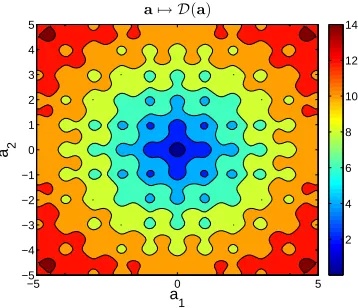
a 1

a 2

a_{7→ D(}a₎

−5 0 5

−5 −4 −3 −2 −1 0 1 2 3 4 5

2 4 6 8 10 12 14

Figure 2: Functiona_{7→ D(}a_{) forN = 2.}

6.1.1 Exact ISDE-based simulated annealing algorithm

For caseN = 2, the ISDE-based simulated annealing sequence, described in Algorithm 2, is generated. The total number of ISDE integrations is nt= 500. For each ISDE, there are Mk = 40 steps. The temperature

decreasing law is chosen as

Tk =T1 exp(−β k) +b. (34)

in which T1 = 36.7,β = 2.0×10−2, b = 3.51×10−2. This function is represented in Fig. 3. To take into

account the constraints, the regularized indicator function in Eq.(20) with α1 =α2 = 0.3. Figure 4 shows

the values A_{1, . . . ,}A_{nt generated using Algorithm 2. It can be seen the capacity of the algorithm to escape}

from local minima and to converge to the global minimum. There are still fluctuations at the end of the simulation since the end-temperature is not zero.

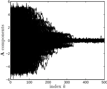
Let’s now increase the dimension toN = 256. The parameter of the temperature decreasing law areT1= 2.5,

β = 2.0×10−2_{, b = 5.1×10}−3_{. Figure 5 shows the valuesA}

1, . . . ,Ant generated using Algorithm 2). It

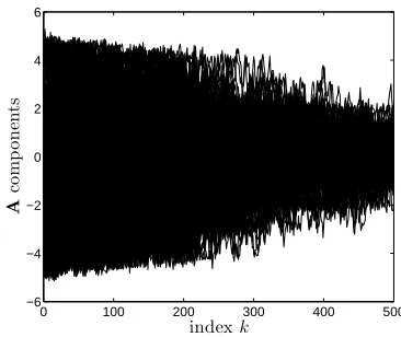
can be seen in this figure that all the components converge to the global minimum. To show the efficiency of this algorithm, these results are compared with the ones obtained using the classical simulated annealing algorithm (1). The same temperature law, and the same increment size calculation method (based on the Hessian of cost function) has been used. Nevertheless, since the calculations of the gradient in Algorithm (2) is more expensive than the simple function evaluations in Algorithm (1), Mk = 170 steps for each MH

0 100 200 300 400 500 5

10 15 20 25 30 35

k_7→Tk

indexk

Tk

Figure 3: Functionk7→Tk.

0 100 200 300 400 500 −6

−4 −2 0 2 4 6

k_7→Ak

indexk

A

k

A

1 k

A

2 k

−6 −4 −2 0 2 4 6 −6

−4 −2 0 2 4 6

Ak

1

A

k 2

Figure 4: ISDE-based algorithm,N = 2, functionsk7→Ak1 andk7→Ak2.

0 100 200 300 400 500 −6

−4 −2 0 2 4 6

indexk

A

co

m

p

o

n

en

ts

Figure 5: ISDE-based algorithm,N= 200, functionsk7→Ak

i fori= 1, . . . ,200.

0 100 200 300 400 500 −6

−4 −2 0 2 4 6

indexk

A

co

m

p

o

n

en

ts

Figure 6: Classical SA algorithm,N= 200, functionsk7→Ak

i fori= 1, . . . ,200.

6.1.2 Approximate ISDE-based simulated annealing algorithm

This section illustrates Algorithm 3 for which the cost function is approximated using a polyharmonic spline approximation at orderp= 2. The initial number of control points isnc= 140. The number of enrichments

isnt= 500. For each ISDE, there areMk= 40 steps. It should be noted that for this simple application the

computation time is larger using the adaptative Algorithm 3 than using the Algorithm 2 (without approx-imation of the cost function). The objective here is just to validate the methodology. The computational gain of Algorithm 3 will be illustrated in the next application which consists in a Finite Element simulation. For case N = 2, Fig. 7 shows the values A_{1, . . . ,}A_{nt. It can be seen again that the algorithm converges}

rapidly to the global minimum. The approximate cost function obtained after the 500 enrichments is plotted

0 100 200 300 400 500 −6

−4 −2 0 2 4 6

k_7→Ak

indexk

A

k

A

1 k

A

2 k

−6 −4 −2 0 2 4 6 −6

−4 −2 0 2 4 6

Ak

1

A

k 2

Figure 7: Approximate ISDE-based algorithm,N = 2, functionsk7→Ak

1 andk7→Ak2.

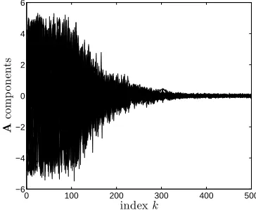
on Fig. 8. Compared with Fig. 2, it can be seen a good approximation of the cost function is the visited regions. For caseN = 32, Fig. 10 shows the valuesA_{1, . . . ,}A_{nt. It can be seen the ability of the algorithm}

to converge to the global minimum when increasing the dimension.

6.2

Finite Element model

We are interested in the maximal response of the 2-storey structure represented in Fig. 10 submitted to the soil acceleration plotted in Fig. 11. This structure is made up with two 3.0×3.0 m2 _{plates (blue color),}

a 1

a 2

a_{7→ D(}a₎

−5 0 5

−5 −4 −3 −2 −1 0 1 2 3 4 5

2 4 6 8 10 12 14 16

Figure 8: Approximate cost functiona_{7→ D}mps_{(a) forN = 2.}

0 100 200 300 400 500 −6

−4 −2 0 2 4 6

indexk

A

co

m

p

o

n

en

ts

Figure 9: Approximate ISDE-based algorithm,N = 32, functionsk7→Ak

i fori= 1, . . . ,32.

by four linear springs. The bottom plate has thickness 5.0×10−3 _{m, Young’s modulus 6.31×10}10 _Pa,

mass density 1800 kg/m3_{, Poisson ratio 0.29. The top plate has thickness 5.0×10}−3 _{m, Young’s modulus}

6.47×1010 _{Pa, mass density 1800 kg/m}3 _{and Poisson ratio 0.29. All the vertical beams have length 3 m,}

diameter 3.5×10−2 _{m (circular section) Young’s modulus 1.3×10}11 _{Pa, mass density 7800 kg/m}3 _and

Poisson ratio 0.3. All the horizontal beams have length 3 m, diameter 3.5 ×10−2 _{m (circular section)}

Young’s modulus 1.3×1011 _{Pa and Poisson ratio 0.3. The north, east, south and west horizontal beams}

have mass density 5800 kg/m3_{, 6800 kg/m}3_{, 7100 kg/m}3 _{and 6800 kg/m}3 _{respectively. The initial value}

for the springs’ stiffnesses (same value for the three directions) are k1 = k2 = k3 = k4 = 70000 N/m.

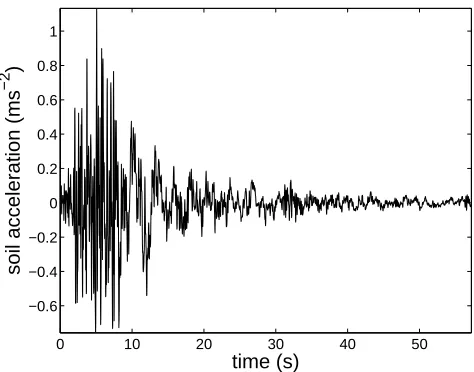
The structure is subjected to the seismic ground acceleration plotted in Fig. 11 along x-direction. We are interested in the displacement at the observation point located at (2,2,2) m on the top plate. The norm of this displacement is plotted in Fig. 12. The objective is to design the stiffnesses of the springs in order to minimize the maximum value of the norm of the displacement. Then a= (k1, k2, k3, k4).To perform this

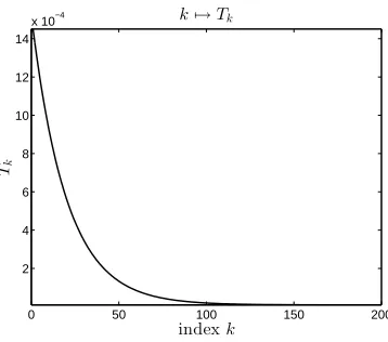
task, the approximated ISDE-based simulated algorithm 3 is used with a polyharmonic approximation at orderp= 2. The admissible domains for the stiffnesses are [5000,120000] N/m. The initial number of control points isnc = 140. The number of enrichments isnt= 200. The number of steps for each ISDE between two

enrichments isMk= 40. The temperature decreasing law is plotted in Fig. 13. The optimal control point is

aopt_{= (19787,18298,59092,70160) N/m. The evolution of the stiffnesses and the exact cost function during}

Figure 10: Finite element mesh.

0 10 20 30 40 50

−0.6 −0.4 −0.2 0 0.2 0.4 0.6 0.8 1

time (s)

soil acceleration (ms

−2

)

Figure 11: Soil acceleration.

0 10 20 30 40 50 0

0.01 0.02 0.03 0.04 0.05

time (s)

displacement (m)

Figure 12: Norm of the displacement at observation point.

0 50 100 150 200 2

4 6 8 10 12 14

x 10−4 k7→Tk

indexk

Tk

Figure 13: Function k7→Tk.

7

Conclusions

0 50 100 150 200 1

2 3 4 5 6 7 8 9 10 11

x 104

index

k

k 1 k

2 k

3 k

4

Figure 14: Evolution of the stiffnesses during the simulation.

0 50 100 150 200

−3 −2.95 −2.9 −2.85 −2.8 −2.75

index

k

co

st

fu

n

ct

io

n

Figure 15: Evolution of the exact logarithm of cost function during the simulation.

References

[Aarts and Laarhoven(1985)] Aarts E. H. L, van Laarhoven P. J. M. 1985. “Statistical cooling: A general approach to combinatorial optimization problems.”Philips Journal of Research 40(4), 193-226.

[Anily and Federgruen(1987)] Anily S., Federgruen A. 1987. “Simulated annealing methods with general acceptance probabilities.”Journal of Applied Probability 24(3) 657-667.

[Azizi and Zolfaghari(2004)] Azizi N., Zolfaghari S. 2004. “Adaptive temperature control for simulated an-nealing: a comparative study.”Computers & Operations Research 31(14), 2439-2451.

2 4 6 8 10 12

x 104 −2.98

−2.96 −2.94 −2.92 −2.9 −2.88 −2.86 −2.84 −2.82

k1

cost function

SPH approximate exact

2 4 6 8 10 12

x 104 −2.98

−2.96 −2.94 −2.92 −2.9 −2.88 −2.86 −2.84 −2.82

k2

cost function

SPH approximate exact

2 4 6 8 10 12

x 104

−2.95 −2.9 −2.85 −2.8 −2.75 −2.7 −2.65

k3

cost function

SPH approximate exact

2 4 6 8 10 12

x 104

−2.95 −2.9 −2.85 −2.8 −2.75 −2.7

k4

cost function

SPH approximate exact

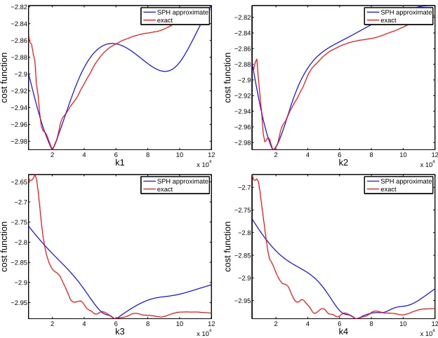
Figure 16: Univariate variations of the exact and approximate logarithm of cost function around the optimal value.

[Borkar(1992)] Borkar V. S. 1992. “Pathwise recurrence orders and simulated annealing.”Journal of Applied Probability 1992, 29(2), 472-476.

[Buhmann(2003)] Buhmann MD. 2003. Radial Basis Functions: Theory and Implementations, Cambridge University Press, New York.

[Burrage(2007)] Burrage K. 2007. “Numerical methods for second-order stochastic differential equation.”

SIAM Journal of Scientific Computing 29(1), 245-264.

[ ˇCern´y(1985)] ˇCern´y V. 1985. “Thermodynamical approach to the traveling salesman problem: An efficient simulation algorithm,Journal of Optimization Theory and Applications 45, 41-51.

[Connors and Kumar(1989)] Connors D. P., Kumar P. R. 1989. “Simulated annealing type markov-chains and their order balance-equations.”SIAM Journal on Control and Optimization 1989 27(6), 1440-1461.

[Duane, et al(1987)] Duane S., Kennedy A. D., Pendleton B. J., Roweth D. 1987. “Hybrid Monte Carlo.”

Physics Letters B 195(2), 216-222

[Faigle and Schrader(1988)] Faigle U., Schrader R. 1988. “On the convergence of stationary distributions in simulated annealing algorithms.”Information Processing Letters 27(4), 189-194.

[Faigle and Kern(1991)] Faigle U., Kern W. 1991. “Note on the convergence of simulated annealing algo-rithms.” SIAM Journal on Control and Optimization 29(1), 153-159.

[Granville, Krivanek, and Rasson(1994)] Granville V., Krivanek M., Rasson J. P. 1994. “Simulated annealing - a proof of convergence.”IEEE Transactions on Pattern Analysis and Machine Intelligence16(6), 652-656.

k1

k2

2 4 6 8 10 12

x 104

1 2 3 4 5 6 7 8 9 10 11 12x 10

4 −2.95 −2.9 −2.85 −2.8 −2.75 k1 k3

2 4 6 8 10 12

x 104

1 2 3 4 5 6 7 8 9 10 11 12x 10

4 −2.95 −2.9 −2.85 −2.8 −2.75 −2.7 −2.65 −2.6 k1 k4

2 4 6 8 10 12

x 104 1 2 3 4 5 6 7 8 9 10 11 12x 10

4 −2.95 −2.9 −2.85 −2.8 −2.75 −2.7 −2.65 −2.6 k2 k3

2 4 6 8 10 12

x 104 1 2 3 4 5 6 7 8 9 10 11 12x 10

4 −2.95 −2.9 −2.85 −2.8 −2.75 −2.7 −2.65 −2.6 −2.55 k2 k4

2 4 6 8 10 12

x 104 1 2 3 4 5 6 7 8 9 10 11 12x 10

4 −2.95 −2.9 −2.85 −2.8 −2.75 −2.7 −2.65 k3 k4

2 4 6 8 10 12

x 104 1 2 3 4 5 6 7 8 9 10 11 12x 10

4 −2.95 −2.9 −2.85 −2.8 −2.75 −2.7 −2.65 −2.6

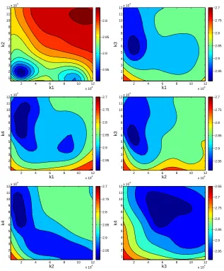
Figure 17: Bivariate variations of the exact logarithm of cost function around the optimal value.

[Hajek(1988)] Hajek B. 1988. “Cooling schedules for optimal annealing.”Mathematics of Operations Research 13(2) 311-329.

[Hastings (1970)] Hastings W. K. 1970. “Monte Carlo sampling methods using Markov Chains and their applications.”Biometrica 109 , 57-97.

[Ingber(1989)] Ingber L. 1989. “Very fast simulated re-annealing.” Mathematical and Computer Modelling

12, 8, 967-973.

[Ingber(1993)] Ingber L. 1993. “Simulated annealing: Practice versus theory.” Mathematical and Computer Modelling 18,(11), 29-57.

[Itˆo(1951)] Itˆo K._{. 1951. “On stochastic differential equations, Memoirs American Mathematical Society 4.}

[Jaynes(1957)] Jaynes E. T. 1957. “Information theory and statistical mechanics.” Physical Review 106(4), 620–630 and 108(2), 171-190.

k1

k2

2 4 6 8 10 12

x 104

1 2 3 4 5 6 7 8 9 10 11 12x 10

4 −2.95 −2.9 −2.85 −2.8 k1 k3

2 4 6 8 10 12

x 104

1 2 3 4 5 6 7 8 9 10 11 12x 10

4 −2.95 −2.9 −2.85 −2.8 −2.75 −2.7 k1 k4

2 4 6 8 10 12

x 104 1 2 3 4 5 6 7 8 9 10 11 12x 10

4 −2.95 −2.9 −2.85 −2.8 −2.75 −2.7 k2 k3

2 4 6 8 10 12

x 104 1 2 3 4 5 6 7 8 9 10 11 12x 10

4 −2.95 −2.9 −2.85 −2.8 −2.75 −2.7 k2 k4

2 4 6 8 10 12

x 104 1 2 3 4 5 6 7 8 9 10 11 12x 10

4 −2.95 −2.9 −2.85 −2.8 −2.75 −2.7 k3 k4

2 4 6 8 10 12

x 104 1 2 3 4 5 6 7 8 9 10 11 12x 10

4 −2.95 −2.9 −2.85 −2.8 −2.75 −2.7 −2.65

Figure 18: Bivariate variations of the approximate logarithm of cost function around the optimal value.

[Kirkpatrick, Gelatt, and Vecchi(1983)] Kirkpatrick S., Gelatt Jr C. D., Vecchi M. P. 1983. “Optimization by Simulated Annealing.”Science 220 (4598), 671-680.

[Kouvelis and Chiang(1992)] Kouvelis P., Chiang W. C. 1992. “A simulated annealing procedure for single row layout problems in flexible manufacturing systems.” International Journal of Production Research

30, 717-732.

[Lundy and Mees(1986)] Lundy M., Mees A. 1986. “Convergence of an annealing algorithm.”Mathematical Programming 34(1), 111-124.

[Mingjun and Huanwen(2004)] Mingjun J, Huanwen T. 2004. “Application of chaos in simulated annealing.”

Chaos, Solitons & Fractals 21, 933-944.

[Mitra, Romeo, and Sangiovanni-Vincentelli(1986)] Mitra D., Romeo F., Sangiovanni-Vincentelli A. L. 1986. “Convergence and finite time behavior of simulated annealing.”Advances in Applied Probability 18(3), 747-77.

0 10 20 30 40 50 0

0.005 0.01 0.015 0.02 0.025 0.03 0.035 0.04 0.045

time (s)

displacement (m)

Figure 19: Norm of the displacement at observation point for the designed structure.

[Pardalos and Romeijn(2002)] Pardalos P., Romeijn E. 2002. Handbook of global optimization, volume 2, Kluwer: Dodrecht.

[Salazar and Toral(1997)] Salazar R., Toral R. 1997. “Simulated Annealing Using Hybrid Monte Carlo.”

Journal of Statistical Physics 89 (5-6), 1047-1060.

[Shannon(1948)] Shannon C. E. 1948. “A mathematical theory of communication.”Bell System Technology Journal 27, 379-423 and 623-659.

[Suman and Kumar(2006)] Suman B., Kumar P. A. 2006. “Survey of simulated annealing as a tool for single and multiobjective optimization.”Journal of the Operational Research Society 57, 1143-1160.

[Soize(1994)] Soize C.. 1994. The Fokker-Planck Equation for Stochastic Dynamical Systems and its Explicit Steady State Solution, World Scientific: Singapore.

[Soize(2008)] Soize C.. 2008. “Construction of probability distributions in high dimension using the maximum entropy principle. Applications to stochastic processes, random fields and random matrices.” Interna-tional Journal for Numerical Methods in Engineering 76(10), 1583-1611.

[Triki, Collette, and Siarry(2004)] Triki E., Collette Y., Siarry P. 2004. “A theoretical study on the behavior of simulated annealing leading to a new cooling schedule.”European Journal of Operational Research

166(1), 77-92.

[Wang, Dong, and Aitchison(2001)] Wang G., Dong Z., Aitchison P. 2001. “Adaptive Response Surface Method - A Global Optimization Scheme for Computation-intensive Design Problems.”Journal of En-gineering Optimization 33, 707-734.

[Yao and Li(1991)] Yao X., Li G. 1991. “General simulated annealing.” Journal of Computer Science and Technology 6(4), 329-338.