A Content-Based Image Retrieval System for Fish Taxonomy

University of New Orleans University of New Orleans

ScholarWorks@UNO

ScholarWorks@UNO

University of New Orleans Theses and

Dissertations Dissertations and Theses

5-22-2006

A Content-Based Image Retrieval System for Fish Taxonomy

A Content-Based Image Retrieval System for Fish Taxonomy

Fei Teng

University of New Orleans

Follow this and additional works at: https://scholarworks.uno.edu/td

Recommended Citation Recommended Citation

Teng, Fei, "A Content-Based Image Retrieval System for Fish Taxonomy" (2006). University of New Orleans Theses and Dissertations. 377.

https://scholarworks.uno.edu/td/377

A CONTENT-BASED IMAGE RETRIEVAL SYSTEM

FOR FISH TAXONOMY

A Thesis

Submitted to the Graduate Faculty of the University of New Orleans in partial fulfillment of the requirements for the degree of

Master of Science in

The Department of Computer Science

by

Fei Teng

B.S, Beijing University of Posts and Telecommunications, 2003

ACKNOWLEDGEMENTS

I would like to thank Dr. Chen for advising me throughout the master’s study. I am

grateful for his continuous help on this thesis. I must also thank Dr. Fu and Dr. Deng for their

TABLE OF CONTENTS

List of Tables………...iv

List of Illustrations………...v

Abstract………...………vi

Chapter 1: Introduction……….………...…....1

Chapter 2: Related work………..3

Chapter 3: Background Knowledge………..………...6

3.1 Image Used………7

3.2 Geometric Morphometrics………..………...8

Chapter 4: Our CBIR System……….………...11

4.1 An Overview of Our System………11

4.2 Feature Extraction...……….14

Chapter 5: Semantic Classification………17

5.1 Binary Classifiers……….………17

5.2 Feature Selection...……….18

5.2.1 Introduction to Supervised Learning and SVM Algorithm………19

5.2.2 SVM Classifier………21

Chapter 6: Similarity Matching……….………24

Chapter 7: Experimental Methods and Results…….………26

7.3.2 Linear Discriminant Analysis (LDA)………32

7.3.3 Boosting………... ……….…………34

Chapter 8: System Interface…..……….………38

Chapter 9: Discussions………..……….39

Conclusion……….41

Reference………...42

LIST OF TABLES

Table1. Features describing shape characters. Non-shape related variation has been removed

from LMi, the landmark coordinates…….……….………..…………..….………..15

Table2. Results from Semantic Classifier based on 2 features ...28

Table3. Results from Semantic Classifier based on 3 features……….….……28

Table4. Results from Semantic Classifier based on 12 features……….……...29

Table5. Results from Linear Regression of an Indicator Matrix………...32

Table6. Results from LDA……….33

Table7. Boosting Classifier to classify C.carpio / the rest……….35

Table8. Boosting Classifier to classify C.cyprinus / the rest……….36

LIST OF ILLUSTRATIONS

Fig.1 Similar images ………..…..………...4

Fig.2 The structure of the CBIR system…………..………...……….5

Fig.3 Ridge ending and ridge bifurcation………..………..…………..……..6

Fig. 4 Images of specimens from three species………..……….7

Fig. 5 Plot of 650 Carpiodes specimens……….………..9

Fig. 6 CBIR Data Flow Diagram………...………12

Fig. 7 Leaning algorithm………..………..13

Fig. 8 A hierarchical classifier for Carpiodes genus………...………...18

Fig. 9 Support Vector Machine………..……….…...20

Fig. 10 SVM maps the data points to a higher-dimensional feature space………21

ABSTRACT

It is estimated that less than ten percent of the world’s species have been discovered and

described. The main reason for the slow pace of new species description is that the science of

taxonomy, as traditionally practiced, can be very laborious: taxonomists have to manually gather

and analyze data from large numbers of specimens and identify the smallest subset of external

body characters that uniquely diagnoses the new species as distinct from all its known relatives.

The pace of data gathering and analysis can be greatly increased by the information technology.

In this paper, we propose a content-based image retrieval system for taxonomic research. The

system can identify representative body shape characters of known species based on digitized

landmarks and provide statistical clues for assisting taxonomists to identify new species or

subspecies. The experiments on a taxonomic problem involving species of suckers in the genera

Carpiodes demonstrate promising results.

Keywords: Content-based image retrieval, shape analysis, feature selection, image classification,

INTRODUCTION

The AI technology can be defined as: attempting to build artificial systems that will

perform better on tasks that humans currently do better [1]. However, since computer is naturally

better than people in the field of processing huge amount of data, AI is becoming more and more

popular today and has expanded from identifying customers by their voices to automatic pattern

classification. Successful retrieval of relevant images from large-scale image collections is one

of the current problems to AI.

One intuitive solution to image retrieval is text-based annotations and indexing. The

indexing process for large image collections is time consuming. Also, text-based indexing for

images only provides hit-or-miss type searching. If the user does not specify the right keywords,

the desired images may be forever unreachable [2]. To overcome these disadvantages,

researchers developed content-based image retrieval (CBIR), which is the set of techniques for

retrieving images from an image database based on automatically-derived image features [3].

This technology can be used to discover unknown species – It is estimated that less than ten

percent of the world’s species have been discovered and described. The main reason for the slow

pace of new species description is that the science of taxonomy, as traditionally practiced, can be

very laborious: taxonomists have to manually gather and analyze data from large numbers of

specimens, often from broad geographic areas, and identify the smallest subset of external body

characters that uniquely diagnoses the new species as distinct from all its known relatives. The

pace of data gathering and analysis in taxonomy can be greatly increased by the development of

information technology. The Internet is being used to link taxonomists, taxonomic literature and

for remote study of specimens archived as digital images. In this thesis, we propose a

content-based image retrieval system for taxonomic research. The system has a learning component that

can identify representative body shape characters of known species based on digitized landmarks.

The system can also provide statistical clues for assisting taxonomists to identify new species or

subspecies. The experiments on a taxonomic problem involving species of suckers in the genera

Carpiodes demonstrate promising results.

The rest of this thesis is organized as follows. In Chapter 2, we introduce related work

done within the field of image retrieval system. Chapter 3 describes the background information

on a taxonomic problem in the fish genus Carpiodes. Chapter 4 introduces the feature extraction

process. Chapters 5 and 6 presents a joint feature selection and classification approach for

semantic classification based on 1-norm support vector machines (SVMs) and a similarity

matching scheme based on the distance in the overall shape space and semantic classification.

Three other classifiers are tested. Chapter 7 demonstrates extensive experiments on a data set of

Carpiodes and discusses the results. Conclusions and possible future work are given in Chapter 7.

Keywords

Content-based image retrieval, shape analysis, feature selection, image classification, taxonomic

Related Work

Image retrieval algorithms roughly fall to two categories, depending on the query format:

text-based approaches and content-based methods. The analysis of user needs in the photo

archives embracing a variety of subject areas (e.g. museums, advertising mass communications)

suggests that text-based methods will remain the basic access method in the foreseeable future

[4]. The text-based approaches are based on the idea of storing a keyword, a set of keywords, or

a textual description of the image content, created and entered by a human annotator, in addition

to a pointer to the location of the raw image data. Image retrieval is then shifted to standard

database management capabilities combined with information retrieval techniques. As pointed

out by Svenonius [27] and Enser [28], text-based retrieval of images is a vicarious access method,

while visual access methods have a high potential to enhance retrieval capabilities.

The main goal of CBIR is to let the computer identify the descriptions of images: high

level concept such as sunset, human or mountain. It leads to a problem: how can the computer

link the nature of digital images, arrays of numbers, to the semantic words? Currently, CBIR

assumes that semantically relevant images have similar visual features, and uses these features,

such as color, texture, and shape to store, identify and search images. This method retrieves

images based on information automatically extracted from pixels. Initially, researchers focused

on querying by image example, where a query image or sketch is given as input by a user [8, 17,

23, 6, 10, 15, 16, 5, 9, 3, 4, 14]. Later systems incorporated feedback from users in an iterative

refinement process [25, 30, 7]. From a computational perspective, a typical CBIR system views

the query image and images in the database (i.e., target images) as a collection of features. It

ranks the relevance between the query and any target image in proportion to a similarity measure

the content of images. And the similarity measure quantifies the resemblance in content features

between a pair of images [21].

This “bridging the semantic gap” (Zhao & Grosky, 2001) problem is considered one of the

greatest challenges to computer vision scientists. Years of experience in the world gives human

beings the ability to distinguish objects -- people exam a picture from several aspects to decide

what it is. A number of general purpose image retrieval engines have been developed, people

still know little about how to effectively and efficiently select and use primitive features to

identify general images. For instance, figure 1 shows that “beach” and “dessert” are viewed

similar by a CBIR system.

(a) (b)

Figure1. Both (a) and (b) are formed by yellow (brown) region and blue region, which makes

them similar to the CBIR system, while actually (a) is beach and (b) is dessert.

In the commercial domain, IBM QBIC [5] is one of the earliest systems. Recently,

additional systems have been developed at IBM T.J. Watson [10], VIRAGE [11], NEC AMORA

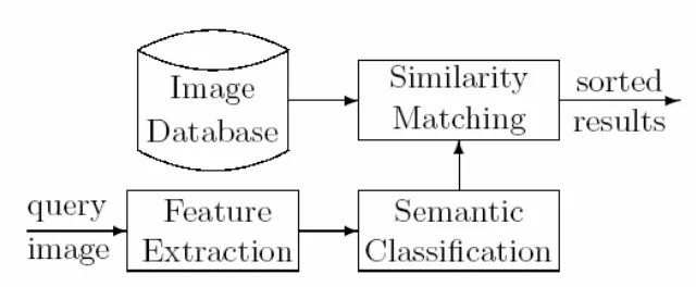
Figure 2: The structure of the CBIR system

However, CBIR is a good solution to specific kind of images, such as medical diagnostics

and fingerprints. Even this kind of pictures is “worse” than ordinary real-life pictures, such as

they often look the same from each others to untrained eyes, this restriction still can effectively

make the algorithm better because:

1. Color is not as important. The color feature can either be treated as discrete values or

colored regions. As shown in Figure1, it is clear that the color feature confuses the

CBIR – if it is understood as discrete values, brown and yellow sand would be identified

different; if it is understood as regions, blue sky and blue water would be identified the

same.

2. Structure of the image is one of the most important features, which makes it possible to

define the features by geometrical functions.

3. The amount of image semantic contents is limited. Figure 3 shows an example of

finger ridges. Representations predominantly based on ridge endings or bifurcations

[31]. Except really special cases, these two classes can represent all kinds of finger

Figure 3: Ridge ending and ridge bifurcation.

A query can be made by an example image and applying partial-match methods to rank retrieved

photos into some calculated similarity order.

So far, CBIR system has been widely utilized in the field of digital forensics, but few

works have been done to apply it to taxonomic research. We know that approximately 1.4

million species are known to science. However, estimates based on the rate of new species

discovery place the total number of species on earth about 10- 30 times of this number. Most

unrecognized species are in poorly studied groups (e.g., insects) occurring in unexplored habitats

(e.g., remote tropical forests). However, a surprising number of new species are still being

discovered in developed countries with long histories of taxonomic research. Human population

expansion and habitat destruction are causing extinctions of both known and yet to be discovered

species. The accelerated pace of species decline has fueled the current biodiversity crisis [18], in

which it is feared that many of the earth’s species will be lost before they can be discovered and

described.

The thesis proposed a CBIR system that can be used to assist taxonomists in discovering

Background Knowledge

1. Dataset

The image database used in this thesis comprises digital photographs of suckers of genus

Carpiodes. However, our approach can be applied to any fish populations. The genus Carpiodes,

as currently recognized, comprises three widely distributed species: the river carp-sucker

Carpiodes carpio (C. carpio); the quillback Carpiodes cyprinus (C. cyprinus), and the highfin

carp-sucker Carpiodes velifer (C. velifer). Figure 4 shows representative images of specimens of

the three species. Most taxonomists regard each of these species as a complex of multiple

biological species in need of revision [24]. The goal of the taxonomic revision in this case is

to identify and formally describe the unrecognized species.

Figure 4: Images of specimens from three species of the genus Carpiodes: C. Carpio, C.

2. Geometric Morphometrics

Over the past decade, geometric morphometric techniques have been developed for

analyzing variation in body shape using a collection of coordinates of biologically definable,

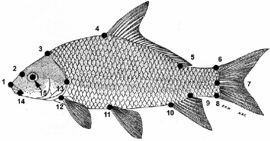
homologous landmarks along the body outline [1]. Figure 5 shows 15 homologous landmarks

digitized on a specimen using the TpsDIG software tool developed by F. James Rohlf of SUNY

Stony Brook2. The analysis methods accompanying the software focus on the landmark

coordinates and geometric information about their relative positions. Through the alignment of

landmarks and statistical analysis of the derived shape variables, groups of specimens may be

identified as distinct in overall shape space. Unfortunately, the current geometric morphometric

methods have two major limitations that hinder successful applications in taxonomic revision

tasks:

• Groups of specimens are distinguished from other populations based on a small set of

derived variables, which are usually functions (in their simplest form, linear

combinations) of all shape variables. As such, derived variables are difficult to

interpret in terms of particular body characters that taxonomists commonly use in

diagnosing new species.

• Shape variation of specimens from closely related species or subspecies may not be

discernible in overall shape space. Therefore, current geometric morphometric methods

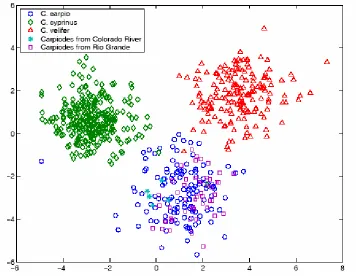
Figure 5: Plot of 650 Carpiodes specimens representing three distinct morphotypes on the first

two canonical variate axes based on derived shape variables from geometric morphometric

analysis of landmark data.

Over the years since [24] was published, Dr. Bart has examined shape and DNA

sequence variation in all Carpiodes populations. Figure 5 shows the results of an analysis of

overall body shape based on a geometric morphometric technique using canonical variate

analysis (CVA). CVA grouped specimens from the Rio Grande (squares), upper Colorado River

(stars), and other western Gulf Slope rivers with C. carpio specimens (circles) from the

Mississippi River Basin. However, a surprising finding from the DNAsequence analysis was that

the forms in Rio Grande and upper Colorado River system of Texas do not agree at all with C.

carpio. Rather, they are closely related to C. cyprinus, which was not known to occur on the

western Gulf Slope. Careful inspection of Carpiodes specimens in the Rio Grande and upper

is diagnostic of C. carpio and C. velifer. They also have a relatively large head and a long snout,

characters seen only in C. cyprinus. However, specimens from these populations also have an

elongate and slender body, and it is these characters that cause them to be erroneously classified

as C. carpio based on overall body shape analysis. It took Dr. Bart three years of careful study of

over 1000 Carpiodes specimens to determine that Rio Grande and upper Colorado River

populations were misdiagnosed as C. carpio, and instead represented a new species related to C.

cyprinus. The question this thesis addresses next is: Can CBIR based on shape features be

applied in a way that diagnoses taxonomic groups in genus Carpiodes more quickly and

The CBIR System

1. An Overview of Our System

The nature of taxonomic research brings the following requirements to the design of an

image retrieval system:

• Text query: Images of specimens from a natural history museum (i.e., the image

database) almost always have textual annotations, e.g., location and date of capture, size

of specimen, species, etc. Therefore, the image retrieval system should support

text-based searches.

• Query by example: A typical usage scenario of the system is to find specimens in the

database that are “semantically similar” to the query specimen based on the query image.

This is clearly a query by example situation. From a taxonomic research point of view,

the image semantics is defined as groupings of related specimens at different

hierarchical levels, which, in the science of taxonomy, are referred to as taxa of varying

rank, i.e., families, genera, species complexes, species, and subspecies.

• Learning component: For the query by example process, the system needs certain

mechanisms to associate feature similarity with semantic similarity, i.e., bridging the

semantic gap. One possible way is to include a learning component capable of

identifying the feature characters that unite populations within each semantic class as

well as distinguishing among semantic classes.

In this thesis, we focus on the CBIR part of the system. Specifically, we propose a

computational framework for categorizing semantic classes of populations based on body shape

the taxonomic research in the following ways:

• It provides taxonomists a tool of efficient searching, browsing, and retrieving images of

specimens archived in natural history museums at distant locations.

• It automatically identifies an “optimal” set of body characters that unites populations

within species, as well as distinguishes among species. Hence it can provide statistical

clues in assisting the discovery of new species or subspecies.

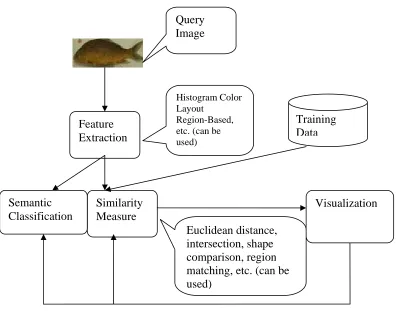
As shown in Figure 6, the system has three major components: Feature Extraction,

Semantic Classification, and Similarity Measure.

Training Data Feature

Extraction

Similarity Measure

Visualization

Histogram Color Layout

Region-Based, etc. (can be used)

Euclidean distance, intersection, shape comparison, region matching, etc. (can be Semantic

Classification

Figure 7: CBIR can be trained by the user

Most learning algorithms should be able to be taught by the user. The CBIR calculates

the similarity between the query image and images in its database, returns the neighbors by the

order of their distances. As shown in figure 7, if the system is given the result 1,2,3,4 and the

user knows that the current answer should be 1,3,2,4, he can tell this to the learning algorithm,

which would learn this issue and rebuild the classifiers. However, this function has not been

realized in our system since a species is just a species. It does not make sense to say that one

velifer is closer to the query velifer than another velifer. CBIR System

Feedback Query

2. Feature Extraction

Figure 6: Digitized 15 homologous landmarks using TpsDIG Version 1.4 (2004 by F. James

Rohlf ).

We focus on the digitized images of specimens with landmarks specified as in Figure 3.

Let LMj, j = 1, · · · , 15, be the coordinates of landmarks on a specimen. We used the technique of

Generalized Procrustes Analysis [12] to remove non-shape related variation in landmark

coordinates. Specifically, the centroid of each configuration (based on the 15 landmarks

associated with each specimen) was translated to the origin, and configurations were scaled to a

common unit size. We computed 12 features, x1, · · · , x12, for each specimen using the 15

• x1–x7: They describe shape characters that can be easily identified visually, for example,

the size of head, the length of body, the distance between the tip of the snout and the

nostril, the size of head in proportion of body size, etc.

• x8–x12: They can be easily evaluated from the landmark coordinates, but may not have a

straightforward visual interpretation. These are the features that a domain expert may

not identify easily, but are candidates of good indicators.

All 12 features were normalized across the specimens via translation and scaling.

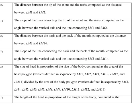
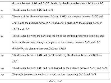
Table 1: Features describing shape characters. Non-shape related variation has been removed

from LMi, the landmark coordinates.

x1 The distance between the tip of the snout and the naris, computed as the distance

between LM1 and LM2.

x2 The slope of the line connecting the tip of the snout and the naris, computed as the

angle between the vertical axis and the line connecting LM1 and LM2.

x3 The distance between the naris and the back of the mouth, computed as the distance

between LM2 and LM14.

x4 The slope of the line connecting the naris and the back of the mouth, computed as the

angle between the vertical axis and the line connecting LM2 and LM14.

x5 The size of head in proportion of the size of the body, computed as the area of the

head polygon (vertices defined in sequence by LM1, LM2, LM3, LM13, LM12, and

LM14) divided by the area of the body polygon (vertices defined in sequence by LM3,

LM4, LM5, LM6, LM7, LM8, LM9, LM10, LM11, LM12, and LM13)

distance between LM1 and LM13 divided by the distance between LM13 and LM7.

x7 The distance between LM7 and LM8.

x8 The sum of the distance between LM3 and LM13, the distance between LM12 and

LM13, and the distance between LM1 and LM13 divided by the distance between

LM13 and LM7.

x9 The distance between the naris and the tip of the snout in proportion to the distance

between the naris and the eye, computed as the distance between LM1 and LM2

divided by the distance between LM2 and LM15

x10 The distance between LM4 and LM11 divided by the distance between LM13 and

LM7.

x11 The distance between LM3 and LM4 divided by the distance between LM13 and LM7.

x12 The angle between the vertical axis and the line connecting LM10 and LM5.

Semantic Classification

1. Binary Classifiers

Semantic classification in our CBIR system targets the following taxonomic problem:

given a collection of labeled specimens (xi' ) represented in a feature space, identify features s

and construct classifiers based on the selected features to distinguish among the known

categories (or species). This problem is closely related to taxonomic revision: if the classifiers

indeed capture the shape properties describing the known species, the classifiers will be helpful

in discovering new species whenever there is shape variation between the new species and all the

known species. For example, if the classifiers assign a group of unlabeled specimens, which are

believed to be taken from the same (but unknown) species, to several known species without a

strong preference on a particular species, it is likely that the unlabeled specimens belong to a

new species in need of description.

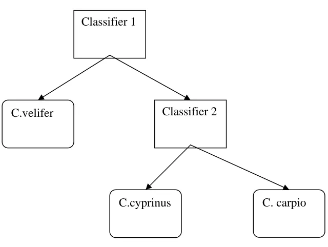
The classification of xiis clearly a multi-class problem. We propose to use a tree

structure to organize binary classifiers into a multi-class classifier. For example, Figure 8 shows

a hierarchical classifier consisting of two binary classifiers for the identification of all three

known species in Carpiodes genus. Finding an “optimal” structure is an interesting research

topic for its own sake, but is beyond the scope of this thesis. Here we assume the structure is

determined beforehand.

For a given collection of samples x_i with the corresponding labelsy_i∈{−1,1}, designing

a binary classifier can be solved by any conventional supervised learning algorithm. However,

we argue that feature selection is indispensable in our system for the following reasons. From a

Figure 8: A hierarchical classifier for Carpiodes genus.

diagnose a species as distinct from its known relatives. The feature selection procedure can

identify those “most” diagnostic features (in this case, body shape characters). From a machine

learning viewpoint, constraining the number of selected features is an effective way to avoid

overfitting. The experimental results in the following section also demonstrate the efficacy of

feature selection in avoiding potential overfitting.

2. Feature subset Selection

Feature subset selection is a well-researched topic in the areas of statistics, machine

learning, and pattern recognition [13, 28]. Existing selection approaches generally fall into two Classifier 1

C.velifer

C.cyprinus

Classifier 2

classification approach. They tend to produce better generalization but may require expensive

computational cost.

2.1 Introduction to Supervised Learning and SVM Algorithm

Supervised learning is a machine learning technique for creating a function from training

data (from Wikipedia.org). The training data consist of vectors (data) and class labels. The

function predicts the value of any valid input object after having learned a number of training

examples. It is a global model that maps input objects to desired outputs.

A support vector machine is a supervised learning algorithm developed over the past

decade by Vapnik and others (Vapnik, Statistical Learning Theory, 1998). SVM algorithm

addresses the general problem of learning to discriminate between positive and negative

members of a given class of n-dimensional vectors [33].

The main idea of this algorithm is to do classification by building a hyperplane in the

N

R space and checking at which side the vector (sample) stays. It can be described as finding a

hyperplane at that space separating the positive from the negative samples. As shown in figure 9,

there may be many separating planes. The statistical learning theory suggests that, for some

classes of well-behaved data, the choice of the maximum margin hyperplane tends to lead to

good generalization when predicting the classification of previously unseen examples (Vapnik,

Statistical Learning Theory, 1998). Sometimes, there is no separating hyperplane, which makes

the “maximum margin” algorithm unusable. Corinna Cortes and Vapnik suggested a modified

idea that allows for mislabeled examples in 1995, which is called soft margin.

-- The margin is understood as the distance from the plane to both classes’ closest data points.

Figure 9: the SVM chooses the plane that maintains a maximum margin from any point in the

training set

This operation may be described by decision functiony=sign(wTx+b), where w is the

vector orthogonal to hyperplane, b is the distance from hyperplane to the origin. In figure 9,

hyperplane A (B) is wTx+b=−1(wTx+b=1). SVM calculates (w,b) from the training data to

achieve the maximum margin 2/w and would like there is no data points between A and B – no

data points between A and B means y(wTx+b)≥1.

Unfortunately, it might be impossible to find a linear solution in the original input space.

The SVM algorithm then uses kernel functions to map the data points to a higher-dimensional

space and find a hyperplane there. Intuitively we can image this transformation would bring Maximum

Margin

Figure 10: SVM maps the data points to a higher-dimensional feature space

The relationship between the kernel function K and the mapping

(.)

φ isK(x,y)=<φ(x),φ(y)>. Intuitively, K(x,y) represents the similarity between x and y. The

great thing here is that we can directly compute K(x,y) without going through the map φ(x),

while the only requirement of this trick is that there is a φ(x) to this kernel.

In many real-world problems such as our CBIR system, the number of negative (positive)

samples is much larger than the number of positive (negative) samples, which would over-train

the classifier – the classifier would treat the weaker class as noise. In our system, we give

different weights to the training data and test data. Also, since our system is a multi-class case

and SVM can only handle one-on-one problem, we use a “one against others” structure as it is

shown figure 8.

2.2 SVM Classifier

The proposed approach is a wrapper model based on 1-norm SVM. Consider the problem

of finding a linear classifier

)

(w x b

sign

y₌ T ₊

where w and b are model parameters. The SVM approach constructs classifiers based on

regularization operator, λ is called the regularization parameter, and erroris commonly defined

through a hinge loss function

} 0 ), (

1

max{ −y wTx+b

= ε

When an optimal solution w is obtained, the magnitude of its component wkindicates the

significance of the effect of the k-th feature on the classifier. Those features corresponding to a

non-zero wk are selected and used in the classifier.

The regularization operator in standard SVMs is the 2-norm of the weight vector w,

which formulates SVMs as quadratic programs (QP). Solving QPs is typically computationally

more expensive than solving linear programs (LPs). SVMs can be transformed into LPs as in

[31]. This is achieved by regularizing with a sparse-favoring norm, i.e., the 1-norm of w,

∑

= _kw_k

w

1

Thus 1-norm SVM is also referred to as sparse SVM and has been similarly applied to other

practical problems such as drug discovery in [2].

Many practical problems in image classification relate to imbalances in samples, i.e., the

number of negative samples is much larger than the number of positive samples. To tackle this

imbalanced issue and make classifiers biased towards the minority class, we penalize differently

on errors produced respectively by positive samples and by negative ones.

Rewrite w_k =u_k −v_k whereu_k,v_k ≥0. If either u_kor v_k has to equal to 0, thenw_k =u_k +v_k.

− + − − + + = − = = +

=

=

≥

=

≥

=

≥

+

+

−

−

=

≥

+

+

−

−

+

+

+

∑

∑

∑

l

j

l

i

d

k

v

u

l

j

b

x

v

u

l

i

b

x

v

u

t

s

l

u

l

u

v

u

,...,

1

,

,...,

1

,

0

,

,...,

1

,

0

,

,...,

1

,

1

]

)

[(

,...,

1

,

1

]

)

[(

.

1

)

(

min

η

ε

η

ε

η

ε

λ

where x i+ and

−

j

x denote a positive sample and a negative sample, respectively, ε and η are

hinge losses, 0 <u < 1 is a constant penalizing the errors from positive and negative samples,

) ( −

+ _l

Similarity Matching

The image similarity measure consists of two parts. The first part corresponds to the

semantic similarity, which is determined by semantic classifier in previous section. If two

specimens belong to the same semantic class, their similarity is the maximum, otherwise the

similarity is zero. Specifically, the semantic similarity between two specimensx _i and x _j is

defined as ⎩ ⎨ ⎧ = otherwise class same the in are x and x x x

s i j i j

0 1 ) , ( 1

The second part reflects the overall shape similarity, and is defined as

2 2

)

,

(

i

x

e

x

s

− −

=

where σ2 is chosen to be the sample variance of the overall shape distance. Note that xi−xj is

the distance in the shape space, hence describes the overall shape difference between two

specimens. The similarity measure is then defined as a convex combination of semantic

similarity and overall shape similarity:

)

,

(

)

1

(

)

,

(

)

,

(

x

x

s

x

x

s

x

x

s

=

α

⋅

+

−

α

⋅

mainly return images that are semantically similar to the query, i.e., specimens in the same group.

Experimental Results

We test the proposed CBIR system on the specimens from the three Carpiodes

morphotypes: C. carpio, C. cyprinus, and C. velifer. The current database contains only 600

images of Carpiodes specimens. However, the proposed computational framework can be

applied to any number of images at any level of fish taxonomy. We are working to expand the

database by including images of specimens of a related group of suckers in the genus Ictiobus.

Our experiment consists of two steps:

• Demonstrating the efficacy of semantic classification by identifying features (or body

characters) for distinguishing among the three Carpiodes morphotypes;

• Applying the system to a taxonomic revision problem involving populations from

Colorado River in Texas and Rio Grande and comparing the results with those based

on the DNA analysis.

1. Experiment based on known fish

The images within each class are randomly divided into a training set and a test set of

equal size. The hierarchical classifier first separates C. velifer-like specimens from specimens of

other species. It then distinguishes C. carpio from C. cyprinus.

We apply the 1-norm SVM to select features and build classifiers simultaneously. The

subspecies.

If the query image is in the training database, the system gives the results by

calculating

s

(

x

,

x

)

=

α

⋅

s

(

x

,

x

)

+

(

1

−

α

)

⋅

s

(

x

,

x

)

If the query image is not in the training database, s₁(x_i,x_j)has to be calculated

byy=sign(wTx+b).

Our proposed algorithm is a wrapper, i.e., the feature selection step is combined with the

classifier. + − − − + − − + + = − = = +

+

=

=

=

≥

=

≥

=

≥

+

+

−

−

=

≥

+

+

−

−

+

+

+

=

∑

∑

∑

l

l

l

l

j

l

i

d

k

v

u

l

j

b

x

v

u

l

i

b

x

v

u

to

subject

l

l

v

u

Z

µ

η

ε

η

ε

η

µ

ε

µ

λ

,...,

1

,

,...,

1

,

0

,

,...,

1

,

0

,

,...,

1

,

1

]

)

[(

,...,

1

,

1

]

)

[(

1

)

(

min

A suitable regularization operator that penalizes large variations of w can reduce

overfitting. In the linear problem above, it makes some of wk =0,k∈[1,12] to do the feature

selection, and it is intuitive that the larger theλ, the fewer features would be selected. There is

no particular way to calculate theλ, we have to try several values to achieve our goals (to select

a certain number of features).

The error rate is defined as the number of misclassified samples over the total number of

Performance based on 2 features:

Table 2: Results from Semantic Classifier based on 2 features

Class Selected Features Training Error Test Error

C.velifer / the rest x₁₀,x₁₁ 10% 11.7%

C.carpio / C.cyprinus x₄,x₇ 12.9% 13.9%

From the results above, we can see that different classifiers need different features (since

we are using a wrapper). The best sub-feature space for distinguishing C.velifer and the rest is

11 10,x

x , and the best sub-feature space for distinguishing C.carpio and C.cyprinus is x₄,x₇.

Performance based on 3 features:

Table3. Results from Semantic Classifier based on 3 features

Class Selected Features Training Error Test Error

C.velifer / the rest x₁₀,x₁₁,x₄ 10.2% 11.8%

C.carpio / C.cyprinus x₄,x₇,x₃ 13.1 % 14%

We observe that the performance based on three selected features is similar to that based

on two selected features. Moreover, we should notice that one more feature does not mean lower

error rates – it may result in larger errors.

Performance based on all features:

C.velifer / the rest All 12 features 8.9% (Linear) 9.8%

C.carpio / C.cyprinus All 12 features 16.5% (Gaussian) 17.3%

Table 4, cont.

From the results above, we can see that all 12 features lead to better performance to

distinguish C.velifer and the rest, but worse performance to distinguish C.carpio and C.cyprinus.

From the results above, we can say that using 12 features cannot guarantee the best result.

However, this conclusion is incomplete since we have not use the classifiers to test suspicious

examples (may be C.velifer, C.carpio, C.cyprinus or other species).

2. Experiment with suspicious fish

Test our CBIR system based on 53 specimens from upper Colorado River in Texas and

the Rio Grande. They were traditionally recognized as C. carpio, yet recent DNA evidence

suggests that both populations are more closely related to C. cyprinus. So we view these 53

specimens as “suspicious” populations. Each “suspicious” specimen is submitted to the system

as a query image. The predicted class label of the query is determined by the majority class

among the top k retrieved images (specimens). We observed that the results are robust for k

varying from 10 to 60. So we pick k = 20. We first set the parameter αin the similarity measure

(1) 0.1. This corresponds to retrieving specimens that are similar to the query based on the

overall shape. It turns out that 52 out of the 53 suspicious specimens are recognized as C. carpio,

and only 1 specimen is identified as C. cyprinus. In other words, the overall shape suggests that

the “suspicious” specimens should be classified as C. carpio. Next, we increase αto 0.9, i.e., the

decision is based mainly on the semantic classifiers. In this case, 23 “suspicious” specimens are

identical results for α= 1.0. Although the hierarchical classifier can distinguish the three species

with reasonable accuracy using only four body shape characters, it has difficulty categorizing the

specimens from Colorado River in Texas and Rio Grande as either C. carpio or C. cyprinus;

43.4% of the “suspicious” specimens are assigned to C. carpio, and 56.6% to C. cyprinus. At the

same time, the retrieved images based on overall shape identify 52 out of 53 specimens as C.

carpio. These contradictory results can be viewed as an indication that the suspicious specimens

represent a new species. It is very interesting that overall shape analysis and the DNA analysis

give similar results: the suspicious specimens are more similar to C. carpio than to C. cyprinus in

terms of the overall shape, yet they are genetically closer to C. cyprinus. Note that our CBIR

system can easily obtain a similar conclusion by adjusting the value of parameter α.

3. Experiment with Suspicious Fish using Other Pattern Classification Techniques

These techniques are different from the algorithm introduced above. They simply build

classifiers that identify all 3 classes simultaneously. We use these classifiers to identify the

suspicious images and evaluate the results. Among the suspicious samples, if

1. None of these percentage values are much larger than the other two or two of them are

much larger than the other one. Since we know these suspicious samples are from one

class, we can make a decision that these fish are not from C.velifer, C.carpio or

C.cyprinus. They are from a new species.

2. One of them is much larger than the other two. Since we know these suspicious

3.1 Linear Regression of an Indicator Matrix

Under the assumption that the decision boundaries are linear, we can consider the

probability of an input x of being classified into class m as fm(x)=βm.0 +βmTx. X would be

labeled as class m if f_m(x)> f_i(x),i=1,...,d, where d is the number of classes. For every two

classes, there is a separating hyperplane in the input space.

The basic idea of is “Linear Regression of an Indicator Matrix” is to code each response

category via an indicator variable. For example, if we have 4 training examples belongs to class

1, 2, 3, 4, the indicator matrix is

⎥ ⎥ ⎥ ⎥ ⎦ ⎤ ⎢ ⎢ ⎢ ⎢ ⎣ ⎡ = 1 0 0 0 0 1 0 0 0 0 1 0 0 0 0 1

Y , then f_m(x)=β_m.0 +β_mTxcan be rewritten as f_m(x)=[1,xT]β_m,

where _m XTX 1XTy_m

)

( −

=

β .

SinceE(Yk |X =x)=Pr(Yk =1|X =x)*1+Pr(Yk =0|X =x)*0=Pr(Yk =1|X =x), we can

simply compute[1,xT]B, whereB=(XTX)−1XTY. The result is a row vector of d elements and

the largest one represents the class on which x lies.

Since the problem is to identify the suspicious images, we use all known images as the

training data and the 53 fish as the test data. Since “Linear Regression of an Indicator Matrix” is

also a linear classifier, we used the features selected for the semantic classifier. Note that these

sub-features may not be the optimal one, but it is a workable one since it is selected linearly. The

results from Linear Regression of an Indicator Matrix are listed below.

Table5. Results from Linear Regression of an Indicator Matrix

C.cyprinus, C.velifer]

were misclassified to

other species.

suspicious fish were

classified to

[C.carpio,

C.cyprinus, C.velifer]

percentage-values of

[C.carpio,

C.cyprinus, C.velifer]

All 12 features [20.31%, 1.68%,

2.32%]

[50, 3, 0] [94.34%, 5.66%, 0]

7 4,x

x [99.22%, 2.02%,

15.12%]

[0, 47, 6] [0, 88.68%, 11.32%]

11 10,x

x [72.66%, 13.13%,

12.21%]

[44, 9, 0] [0, 83.02%, 16.98%]

11 10 7 4,x ,x ,x

x [28.90%, 3.37%,

5.23%]

[45, 8, 0] [0, 84.91%, 15.09%]

Table 5, cont.

From this table, we can observe:

1. Using 12 features, the classifier is not good at identifying C. carpio and identifies the 53 fish

as C.carpio..

2. The classifier gives totally different result with different feature selection.

Given the result that the suspicious fish are from a new species, we know that Linear

distributions are Gaussian densities ∑ = = − − −

∑

π and all classes

have a common covariance matrix, we can say that the decision boundary between any two

classes is a hyperplane. These linear discriminant functions

are log ( )

2 1 )

(x x 1 1 p k

f T _{k k}T _k

k =

∑

∑

) ( ) ( ) ( 2 1 ) ( ) ( log ) | Pr( ) | Pr(

log 1 1 k j

T j k T j k x j p k p x X j G x X k G µ µ µ µ µ µ + − + − − = = = = =

∑

∑

In the class conditional distributions, we can estimate the mean vector as

∑

= = k g i k k i x N 1

µ . The

covariance matrix is estimated as

∑

∑

∑

= = − − − = k g T k i k i K k i K N x

x )( ) /( )

(

1

µ

µ . p(k)=Nk/N

Since the problem is to identify the suspicious images, we use all known images as the

training data and the 53 fish as the test data. Since this classifier is not time-consuming, we tried

all combinations of any 2 features to achieve the best result. The results from Linear Regression

of an Indicator Matrix are listed below.

Table6. Results from LDA

Class Selected Features Training Error Test Error Suspicious Fish

C.velifer / the rest x₁₀,x₂ 6.0% 8.6% 0 velifer

C.carpio / C.cyprinus x₁,x₇ 10.3% 20.1% 21 Cyprinus, 31 Carpios

C.velifer / the rest All 12 features 5.1% 8.0% 0 velifer

Same as the semantic classification, the classifier identifies the suspicious fish as a new species if

we select features. With all 12 features, the LDA classifies most of the samples to carpio.

Furthermore, as we tried different training/test bipartitions, the LDA selected different

sub-features to achieve the best result. We observe that feature 10 will always be used to distinguish

velifer/ the rest and feature 7 will always be used to distinguish carpio/cyprinbus.

3.3 Boosting

Boosting was formulated based on an interesting result from machine learning: learners,

each performing only slightly better than random guess (“week learners”), can be combined to

form an arbitrary “strong” classifier.

The AdaBoost algorithm is:

Given training data (x1,y1),...,(xm,ym)wherexi∈X,yi∈{1,−1}. InitializeD1(i)=1/m,

For t=1,…,T

1. Train weak learner h1:X->{1,-1} using distribution Dt.

2. Compute error

∑

≠

=

i i

t x y

h i

i

t D i

) ( : ) ( ε

3. Choose ln(1 )

2 1 t t t _ε ε α = − 4. Update ⎪⎩ ⎪ ⎨ ⎧ ≠ = = ₋ + i i t i i t i t t y x h e y x h e Z i D i D t t ) ( ) ( * ) ( ) ( 1 _α α

, where Ztis a normalization factor (chosen so

step 3, we can observe that a smaller error corresponds to a largerαt, which means a stronger

weaker classifier is “heavier” in the final decision. Also, in each round, step 4, the sample

distribution is also updated. The weights for all misclassified samples are increase, while the

weights for the rest samples are reduced. Intuitively, the misclassified samples will receive

higher attention in the next learning iteration.

This algorithm will generate 3 relatively good classifiers from the weak LDA classifier.

Each classifier can only recognize one class (one against others).

The first one is to distinguish C.carpio / the rest

Table7. Boosting Classifier to classify C.carpio / the rest

Selected Features Training Error

[t=1,…,t=10] (%)

Test Data

(with best T)

[C. carpio, the rest]

Percentage-values of

[C.carpio, the rest]

All 12 features [14.91, 7.70, 5.86,

6.03, 6.36, 6.19, 6.03,

6.19, 6.19, 6.19]

[53, 0] [100%, 0]

7 1,x

x [21.44, 20.26, 11.39,

11.39, 9.38, 9.04,

9.21, 9.04, 9.04,

9.04]

[26,27] [49.06%, 50.94%]

2 10,x

x [17.42, 10.05, 10.72,

9.55, 8.37, 8.04, 8.04,

8.04, 8.04, 8.04]

Following is the classifier 2, which identifies C.cyprinus / the rest.

Table8. Boosting Classifier to classify C.cyprinus / the rest

Selected Features Training Error

[t=1,…,t=10] (%)

Test Data

(with best T)

[C. carpio, the rest]

Percentage-values of

[C.carpio, the rest]

All 12 features [2.68, 1.67, 1.34,

1.17, 1.17, 1.17, 1.34,

1.34, 1.34, 1.34]

[41, 12] [77.36%, 22.64%]

7 1,x

x [7.53, 6.70, 6.53,

6.03, 6.03, 6.19, 6.19,

6.19, 6.19, 6.19]

[25, 28] [47.17%, 52.83%]

2 10,x

x [25.29, 25.46, 25.12,

24.28, 2.84, 2.84,

2.84, 2.84, 2.84,

2.84]

[25, 28] [47.17%, 52.83%]

Following is the classifier 2, which identifies C.cyprinus / the rest.

Table9. Boosting Classifier to classify C.velifer / the rest

Selected Features Training Error

[t=1,…,t=10] (%)

Test Data

(with best T)

Percentage-values of

4.18, 4.18, 3.85]

7 1,x

x [28.98, 25.63, 22.45,

16.75, 17.76, 17.92,

17.76, 17.76, 17.76,

17.59]

[30, 23] [56.60%, 43.40%]

2 10,x

x [12.73, 13.40, 11.55,

11.72, 11.56, 11.39,

11.39, 11.39, 11.39,

11.39]

[0, 53] [0, 100%]

Table 9, cont.

The classifiers achieved totally different results with different feature selections.

However, since the features we used are from a wrapper feature selection algorithm, the result

with 12 features is more reliable. From classifier C.carpio / the rest, we know that 100%

suspicious fish are from C.carpio. From classifier C.cyprinus / the rest, we know that 77.36%

suspicious fish are from C.cyprinus. From classifier C.velifer / the rest, we know that none of the

suspicious fish are from C.velifer. The contradictory from the first 2 classifiers and classifier 3’s

System Interface and Conclusion

1. System Interface

The system has a simple CGI-based query interface. Users can either enter the ID of an

image as the query or submit any image (along with a file containing the landmarks) via the

Internet. Figure 6 shows the 25 thumbnails returned by the system where the query image (C.

Cyprinus) is on the top left. The parameter αin (1) was chosen to be 0.8. Below each thumbnail

are image ID and the name of its taxonomic category. Users can start a new query search by

submitting a new image ID or image files.

section. We tested two classifiers, namely, linear SVM and SVM with Gaussian kernel. All the

classifiers were constructed using half of the 600 specimens and tested over the remaining 300

specimens. The 12-feature classifiers generate significantly different predictions on the 53

“suspicious” specimens from the selected-feature classifiers. Both classifiers assign the majority

of the 53 specimens to C. carpio, which contradicts the results generated by 1-norm SVM. An

interesting question arises: which results should we trust, those based on the selected features or

those using all the features? We argue that feature selection is indispensable for the following

reasons:

• From a taxonomic viewpoint, it is desirable to use a small number of body shape

characters to describe a species as distinct from its known relatives. The feature

selection procedure can identify those “most” diagnostic features (or body shape

characters).

• From a machine learning viewpoint, constraining the number of selected features is an

effective way to avoid overfitting. One may reason that the above conflicting result for

Colorado River and Rio Grande specimens is due to overfitting, i.e., the models trained

on all 12 features overfit the data.

For the other 3 pattern classification techniques, Linear Regression of an Indicator Matrix and

Linear Discriminant Analysis (LDA) do not work well on this problem. AdaBoost is good at

improving the performance of LDA and produced a classifier that can identify all four classes

(C.carpio, C.cyprinus, C.velifer and suspicious fish) correctly with 12 features. However, since

“from a taxonomic viewpoint, it is desirable to use a small number of body shape characters to

describe a species as distinct from its known relatives”, we cannot say that it will work on more

3. Thesis Conclusion

In this thesis, we proposed a content-based image retrieval approach for taxonomic

research. The system has a learning component that automatically identifies the semantic class of

a query based on digitized landmarks. We applied the system to a taxonomic problem in genus

Carpiodes. The results are promising: the proposed framework not only learned classifiers that

well separated the three known species in Carpiodes using only a few body shape features, but

also recognized “suspicious” specimens that could not be identified previously without the aid of

DNA analysis. Therefore, our framework provides a powerful tool for assisting the diagnosis of

new species and increasing the pace of taxonomic research. As continuations of this work,

several directions may be pursued. Our system can be linked to the Internet so that taxonomists

around the globe can not only retrieve specimens from the system, but can contribute images to

expand the database. The learning component in the system can potentially be extended to any

taxonomic problem involving a large data set and a significant percentage of unknown

specimens in a semi-supervised learning framework. An important future direction of this

References

[1] Robert Wray, Ron Chong, Joseph Phillips, Seth Rogers, and Bill Walsh, “A Survey of

Cognitive and Agent Architectures”, Winter 94

[2] J. R. Smith, S.F. Chang, “Tools and Techniques for Color Image Retrieval,” Proc.

IS&T/SPIE Storage & Retrieval for Still Image and Video Databases IV, San Jose, CA, Feb.,

1996, pp. 426-437.

[3] James Z. Wang, Jia Li, Gio Wiederhold, “SIMPLIcity: Semantics-sensitive Integrated

Matching for Picture Libraries” IEEE Trans. on Pattern Analysis and Machine Intelligence,

vol 23, no.9, pp. 947-963, 2001

[4] E. Sormunen, M. Markkula and K. Jarvelin, “The Perceived Similarity of Photos - A

Test-Collection Based Evaluation Framework for the Content-Based Image Retrieval Algorithms”,

MIRA '99 Glasgow, Scotland, 14th-16th April 1999

[5] M. Flickner, H. Sawhney, W. Niblack, J. Ashley, Q. Huang, B. Dom et al. “Query by Image

and Video Content: The QBIC System”, IEEE Computer, vol. 28, no. 9, 1995.

[7] Gong Y., “Intelligent image databases : towards advanced image retrieval”, Boston, Kluwer

Academic Publishers, 1998.

[8] Gudivada VN, Raghavan VV. “Modeling and retrieving images by content.” Information

processing & Management, 33(4):427-452, 1997

[9] Gupta A, Jain R. “Visual information retrieval”, Communications of the ACM, 40:71-79,

1997.

[10] J.R. Smith and C.S. Li, “Image Classification and Querying Using Composite Region

1999

[11] International Code of Zoological Nomenclature, 4th edition. International Trust for

Zoological Nomenclature, c/o Natural History Museum, 1999

[12] D. G. Kendall, “Shape-manifolds, procrustean metrics and complex projective spaces.”

Bulletin of the London Mathematical Society, 16:81-121, 1984

[13] R. Kohavi and G. H. John, “Wrappers for feature subset selection”, Artificial Intelligence,

97(1-2):273-324, 1997.

[14] J. Li and J. Z. Wang, “Automatic linguistic indexing of pictures by a statistical modeling

approach.” IEEE Trans. Pattern Analysis and Machine Intelligence, 25(9):1075-1088, 2003.

[15] W. Y. Ma and B. Manjunath, “NeTra: a toolbox for navigating large image databases.” In

Proc. IEEE Int’l Conf. on Image Processing, pages 568-571. 1997

[16] S. Mehrotra, Y. Rui, M. Ortega-Binderberer, and T. S. Huang, “Supporting content-based

queries over images in MARS” In Proc. IEEE Int’l Conf. on Multimedia Computing and

Systems, pages 632-633. 1997

[17] A. Pentland, R. W. Picard, and S. Sclaroff, “Photobook: content-based manipulation for

image databases.” International Journal of Computer Vision, 18(3):233-254, 1996.

[18] S. L. Pimm and J. H. Lawton, “Ecology–planning for biodiversity.” Science, 279:2068-2069,

1998.

[19] J. E. Rodman and J. H. Cody, “The taxonomic impediment overcome: NSF’s partnerships

[21] S. Santini and R. Jain, “Similarity measures” IEEE Trans. Pattern Analysis and Machine

Intelligence, 21(9):871-883, 1999.

[22] A. W. M. Smeulders, M. Worring, S. Santini, A. Gupta, and R. Jain, “Content-based image

retrieval at the end of the early years” IEEE Trans. Pattern Analysis and Machine

Intelligence, 22(12):1349-1380, 2000

[23] J. R. Smith S.F. Chang, “VisualSEEK a fully automated content-based query system” In

Proc. 4th ACM Int’l Conf. on Multimedia, pages 87-98. 1996.

[24] R. D. Suttkus and H. L. Bart, Jr., “A preliminary analysis of the river carpsucker, Carpiodes

Carpio, in the southern portion of its range.” In L. Lozano (ed.) Libro jubilar en honor al Dr.

Salvador Contreras Balderas, Universidad Autonoma de Nuevo Leon, Monterrey Mexico,

pages 209-221. 2002.

[25] S. Tong and E. Chang, “Support vector machine active learning for image retrieval” In Proc.

9th ACM Int’l Conf. on Multimedia, pages 107-118. 2001.

[26]Enser PG, “Pictorial information retrieval” Journal of Documentation 51, pages 126-170,

1995

[27] Q. D. Wheeler, P. H. Raven, and E. O. Wilson. “Taxonomy: impediment or expedient?”

Science, 303:285, 2004

[28] L. Yu and H. Liu, “Efficient feature selection via analysis of relevance and redundancy”

Journal of Machine Learning Research, 5:1205-1224, 2004

[29] M. Zelditch, D. Swiderski, D. Sheets, and W. Fink, “Geometric Morphometrics for

Biologists: a Primer.” Elsevier Academic Press: London, 2004.

[30] X. S. Zhou and T. S. Huang, “Comparing discriminating transformations and SVM for

137-146, 2001

[31] J. Zhu, S. Rosset, T. Hastie, and R. Tibshirani, “1-norm support vector machines” Advances

in Neural Information Processing Systems, 16. 2004

[32] A. K. Jain and S. Pankanti, “Fingerprint Classification and Matching”, Handbook for Image

and Video Processing, A. Bovik (ed.), Academic Press, April 2000.

[33] Li Liao, William Stafford Noble, "Combining pairwise sequence similarity and support

vector machines for remote protein homology detection", The Proceedings of The Sixth

International Conference on Research in Computational Molecular Biology (RECOMB

Vita

Fei Teng was born in Tianjin, China. With years of hard work like many other Chinese

students did, he was admitted to Beijing University of Posts & Telecommunications, one of the

top Chinese universities. He received his Bachelor’s Degree in Computer Science & Technology

in 2003. He worked 1 year as an assistant engineer in China Netcom Group, Beijing

Communications Corp. in the capital of China, Beijing.

He began his graduate study in Computer Science at University of New Orleans in Spring

2005 and worked as a graduate assistant under Dr.Yixin Chen.

In the spare time, he likes reading and traveling. He has great interests in history and